

Bolt has demonstrated that a shared scooter can be more than a vehicle. It can also be a mobile geospatial sensor.
During its Wheels4Wheels pilot in Tallinn, Estonia, the company used sensors already installed in its scooters to assess pavement conditions, curb transitions and other features affecting wheelchair users and people with reduced mobility.
Bolt says the project covered approximately 550 kilometres across all eight Tallinn districts, producing 40.5 million accelerometer readings and more than 66,000 surface-quality assessments. The resulting information was contributed to OpenStreetMap, according to Bolt’s accessibility programme page.
Publishing the results as open data makes the project more significant than a conventional corporate mapping exercise. Municipalities, routing applications and accessibility services could all potentially use the observations.
The larger opportunity is the conversion of commercial vehicle fleets into continuously operating urban-observation networks. Thousands of scooters already traverse city streets during everyday operations, potentially detecting damaged surfaces and deteriorating infrastructure without requiring a dedicated municipal survey.
According to Geo Week News, Bolt combined GPS with accelerometers, gyroscopes and cameras. The company reports that the pilot increased available surface-quality data in Tallinn by 26%. These figures have not been independently audited.
The difficult step is converting motion signals into reliable accessibility information. A vibration could represent broken pavement, cobblestones, a drainage channel or an abrupt rider manoeuvre. Results may also vary with speed, tyre pressure, weather and scooter model.
Coverage presents another limitation. Scooters primarily travel where their use is permitted and commercially viable. They may miss residential streets, pedestrian paths and disconnected sections that create the greatest problems for wheelchair users.
Each observation therefore needs provenance, a confidence level and an effective validation method. The most important validators should include wheelchair and mobility-aid users, who can determine whether a detected anomaly represents a genuine barrier.
Wheels4Wheels complements rather than replaces existing accessibility platforms. Wheelmap maps the accessibility of public places, while Project Sidewalk combines crowdsourcing, machine learning and street imagery to identify curb ramps and obstacles. Bolt adds passive, recurring fleet sensing.
A future workflow could use scooter telemetry to flag anomalies, imagery to classify them and local contributors to confirm their significance before the information enters OpenStreetMap.
Public discussion of the project has also highlighted a contradiction: poorly parked scooters can themselves block sidewalks and curb ramps. Bolt’s accessibility strategy must therefore address parking and obstruction management alongside data collection.
If the company can demonstrate reliable classification, transparent data handling and meaningful participation by accessibility users, Wheels4Wheels could evolve into more than a mapping experiment. The sensing capacity already exists. The next challenge is turning it into trustworthy, routable and genuinely inclusive geospatial infrastructure.


#GeoAI


Next article
The Superspectral Shift: Why the Remote Sensing World Is Moving Away from Old Multispectral Limits

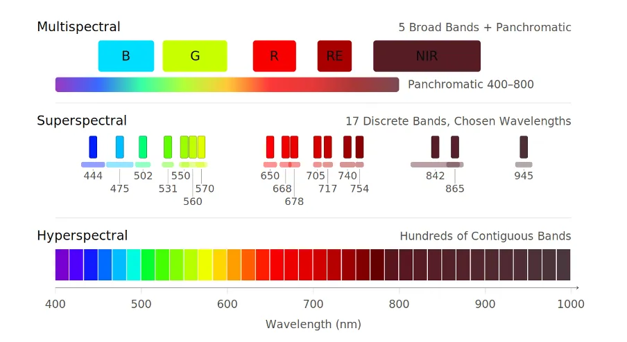
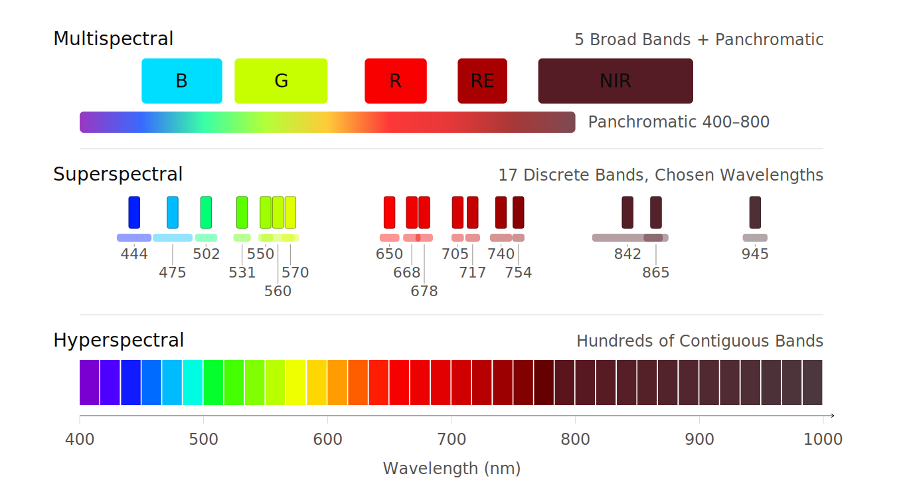
For decades, “more bands” in Earth observation meant one of two things: you either work with multispectral sensors; four to ten broad bands, cheap, fast and familiar or else transition to the hyperspectral domain, which has hundreds of narrow, contiguous bands, costly and enormous data volumes. However, this gap is closing not by making hyperspectral high-resolution accessible, but by rethinking what “enough bands” actually means. A category is quietly establishing itself between the two: Superspectral, a curated set of roughly a dozen to a few dozen discrete bands, placed purposely at specific wavelengths that correspond to something physically meaningful, rather than being sampled continuously across the electromagnetic spectrum.
The Multispectral Ceiling
Multispectral sensors were built around a simple idea: a handful of broad bands such as blue, green, red, red-edge, near-infrared are enough to compute NDVI & NDRE, delineate landcover, and monitor vegetation vigour at scale. Many of these systems also carry a panchromatic band: a single high-resolution spectral channel spanning across the visible spectrum (400-800 nm), used purely to sharpen spatial detail rather than to add spectral information. That’s the multispectral-era trade-off at minimal where spatial resolution and spectral resolution were treated as two separate problems, solved by two different types of bands. It works and it still works, for a huge share of remote sensing applications.
However, broad bands average out the very features that distinguish stressed vegetation from healthy vegetation, one water body from another, or one mineral from the next. A 100-120 nm wide band cannot resolve a narrow absorption or reflectance feature within it. Indices tied to specific physiological or physical processes such as pigment ratios, early-stage stress signatures and water turbidity, often require reflectance captured at precise, narrow wavelengths which a standard four or five-band setup was never designed to capture.
Why Hyperspectral isn’t the Universal Answer
Hyperspectral imaging solves the problem by capturing contiguous and narrow bands. A 20-band sensor covering 500-700 nm at 10 nm interval is hyperspectral by this definition, while a sensor with 20 discrete, non-adjacent bands spanning the visible through infrared is still, technically a multispectral. That distinction matters because hyperspectral sensors carry real expense; complex optics, strict calibration requirements, and data volumes that stretch onboard storage, downlink bandwidth, and downstream ML pipelines. For most applied problems, that’s more data than the underlying problem statement actually needs.
The Middle Category: Superspectral
Superspectral fits between the two. Rather than sampling the electromagnetic spectrum continuously, it samples it selectively – a dozen-plus discrete, narrow bands chosen because they align with known absorption or reflectance features, not because they happen to be adjacent on a continuum. It’s a knowledge-first approach to sensor design: instead of asking “how much of the spectrum can we cover continuously,” it asks “which specific wavelengths actually carry the signal we care about.”
This only works if the band selection is grounded in the underlying physics or biology of the target. Which is exactly where the reasoning gets interesting — because the “right” dozen bands look completely different depending on what you’re trying to measure.
Building the Case: Three Domains, Three Different Superspectral Stacks
- Coastal & Aquatic — A dedicated coastal-blue region
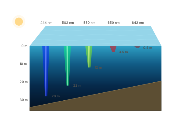
Water quickly absorbs longer wavelengths, which is exactly why coastal and bathymetric applications require the shorter wavelength of the visible spectrum. In clear, deep water 400-450 nm wavelength penetrates furthest, making it the band of choice for shallow-water bathymetry and seafloor mapping. In turbid or CDOM-rich coastal water the picture inverts: suspended sediment and dissolved organic matter absorb and scatter strongly in the blue, and the transmission peak migrates toward green. On sediment loaded reef sites it has been observed shifting by around 100 nm into the green-yellow, peaking near 575 nm. A standard multispectral blue band, which is broadly tuned for atmospheric correction and land applications, is not optimized for this; a narrow, purpose-placed coastal-blue bands are. This is a case where one extra, carefully positioned band is more beneficial for the application than several additional generic ones.
- Agriculture & Forestry — How discrete spectral selection works?
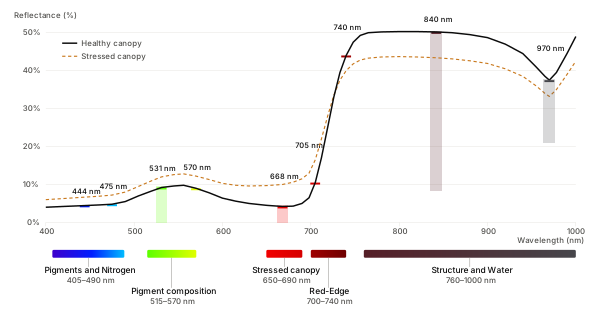
- Green/yellow region (515–570 nm): Chlorophyll absorption is weak in the region, so carotenoids and anthocyanins dominate the signal, and small changes in the pigment show up as measurable changes in reflectance. Photochemical Reflectance Index (PRI), which pairs a band at 531 nm tracking the xanthophyll cycle, the fast photoprotective response of the canopy against a reference band near 570 nm where that cycle has no effect. The 531/570 pairing is the clearest illustration in the whole vegetation stack of why discrete placement matters, a single broad green band averages both of them into one number that carries neither.
- Red region (650–690 nm): Tracks pigment concentration, with the chlorophyll absorption maximum near 670-680 nm. When, paired with the red-edge bands, it helps constrain the shape of the absorption feature rather than just its depth. At 687 nm band, it allows retrieval of solar-induced chlorophyll fluorescence, a direct proxy for photosynthetic activity rather than just the presence of pigment.
- Red-edge region (700–750 nm): The single most diagnostic region for vegetation stress. Healthy vegetation shows a redshift (the edge moves toward NIR); stressed or drought-affected vegetation shows a blueshift. This one narrow region does more stress-detection work than broad NIR alone ever could.
- NIR region (780–1000 nm): Reflectance is dominated by scattering, not absorption; biomass, leaf area index, and water absorption through near 970 nm that supports biochemical property retrieval independent of pigment signals.
- Urban — Where the same spectral logic becomes more conditional.
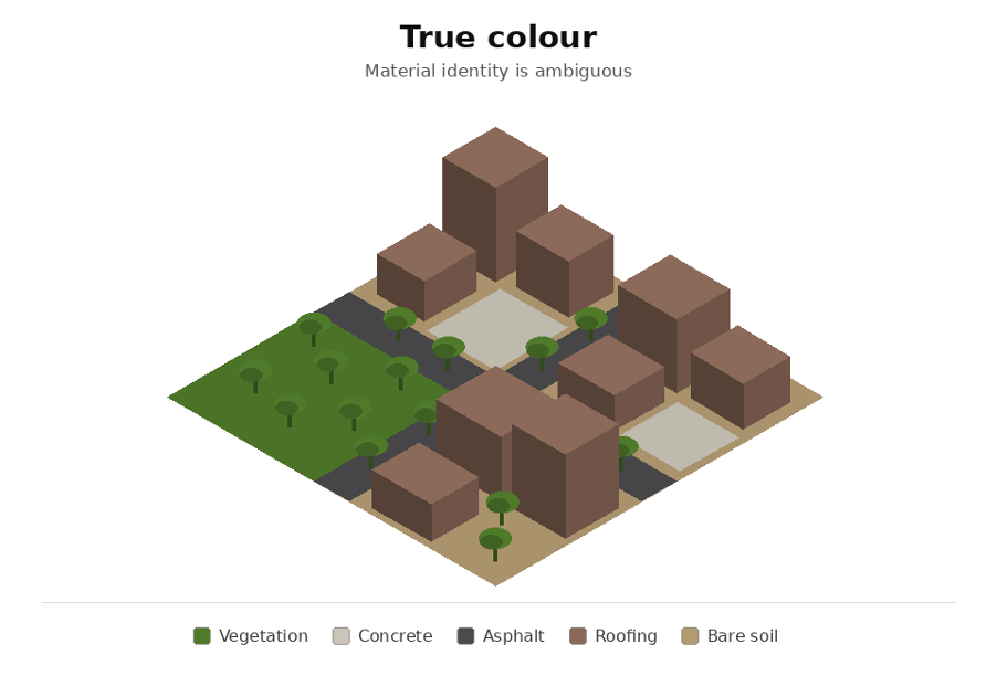
Extending the vegetation logic straight into urban environments using Red-edge and NIR bands, but the physics doesn’t transfer as cleanly. Red-edge and NIR bands are diagnostic of chlorophyll and canopy structure, which makes them excellent for mapping urban vegetation fraction: street trees, park canopy, green-roof coverage, and green-space stress, all of which are legitimate and useful urban indicators, especially as proxies for urban surface extent and heat island risk. But Red-edge and NIR bands are not, a strong basis for classifying built materials themselves — asphalt, concrete, and rooftops don’t have a red-edge-style feature the way vegetation does. The spectral region that most cleanly separates impervious surfaces from vegetation and bare soil sits further out, in the shortwave infrared, where built materials and natural surfaces diverge most sharply. A Red-edge/NIR-only superspectral stack can tell you a great deal about a city’s green infrastructure; it can’t, tell you what the non-green parts of the city are made of. Getting that requires extending the band selection into SWIR — which is a fair, extension of the same superspectral principle: add exactly the band the physics calls for, nothing more.
Superspectral Sensors Exists: Drones to Satellites
Micasense Drone payload: RedEdge-P Triple. A stacked triple narrowband camera bodies on one drone platform, each contributing a handful of 15 discrete, narrow, non-contiguous bands, pan-sharpened to 4 centimetres per pixel, enough to compute pigment and stress-sensitive indices that a standard five-band multispectral sensor can’t generate. This is the smallest-scale, most accessible end of the superspectral sensor; no continuous spectral coverage, just a deliberately chosen set of narrow bands.
Commercial VHR satellite: WorldView-3. Launched in 2014, WorldView-3 is explicitly described in the remote sensing literature and by its operators as a “Superspectral” sensor, a term used specifically to distinguish it from hyperspectral. Its imager collects 8 discrete VNIR bands (coastal, blue, green, yellow, red, red-edge, and two NIR bands), 8 discrete SWIR bands, and a separate 12-band CAVIS instrument for atmospheric correction (clouds, aerosols, water vapor, ice, and snow) 29 bands in total, but none of them contiguous in the way a hyperspectral band are. That distinction matters: WorldView-3 has been used for tasks like hydrocarbon and mineral detection that’s the domain of hyperspectral, precisely because its SWIR bands were placed at known diagnostic absorption features rather than spread evenly across the spectrum.
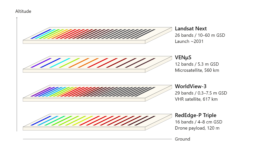
Research microsatellite: VENμS. A joint French–Israeli mission (CNES and the Israel Space Agency, launched 2017), was purpose-built VENμS Super-Spectral Camera (VSSC) with exactly 12 narrow bands between 415–910 nm, at 5.3 m resolution with a 2-day revisit. The band placement was designed specifically around vegetation status and the chlorophyll red-edge, plus atmospheric correction. It’s one of the cleanest real-world matches to the “12-18 narrow, targeted bands” definition of superspectral, since it was purpose-built as a science mission rather than adapted from a broader commercial sensor.
Next-generation Landsat constellation: Landsat Next. Planned for launch in late 2030/early 2031, the USGS and NASA’s Landsat Next mission is explicitly presented as “26-band Superspectral”, more than double the 11 bands on Landsat 8 and 9. It combines refined versions of Landsat’s legacy bands, ten new bands targeting applications like harmful algal blooms and snow hydrology, and five thermal infrared bands. When, a government agency formally classifies its flagship imaging mission as “superspectral” rather than multispectral or hyperspectral, that’s a strong indication the category has moved from marketing language to an accepted technical classification.
Why This Matters for GeoAI Pipelines
The pattern across all three domains is the same, and it’s the real reason for superspectral as a category:
- Information density over band count. A dozen bands selected against known absorption features carry more discriminative signal per band than a broader, generic stack, without the storage and preprocessing burden of a full hyperspectral cube.
- Physics-informed feature engineering. Bands chosen for red-edge stress detection, coastal water penetration, or pigment-specific absorption effectively encode domain knowledge directly into the input, reducing how much a downstream model has to learn from raw reflectance alone.
Where This Is Headed: Future
The multispectral or hyperspectral is a simple binary choice. Superspectral won’t replace either, broadband multispectral remains the workhorse for large-scale, low-cost monitoring, and hyperspectral remains necessary where continuous spectral coverage matters, like detailed mineral mapping or ore detection. But for the growing set of problems that need specific physical or biological signals – water quality, vegetation stress, urban green infrastructure and many more; without the overhead of a full hyperspectral sensor system, superspectral is becoming the realistic answer. It’s less “how much of the spectrum can we see” and more “how much do we actually need to see, and where.”
Superspectral systems, by design, only see what they were told to look for. That’s a real trade-off, not a compromise to gloss over, it’s the whole point of this technology.