
For many GIS teams, spatial data still begins in a database. Parcels, roads, buildings, utility networks, and field edits are stored, checked, and served from systems that many people can use at the same time. In this world, PostGIS became one of the most trusted foundations for operational GIS.
That role is still important. PostGIS is excellent when the task requires live multi-user editing, strict spatial constraints, and safe, concurrent transactions. It helps teams maintain authoritative data and serve low-latency spatial queries to applications. If a city is editing road closures or a utility company is updating pipe networks, PostGIS is still a strong choice.
But analytical GIS has a different shape. It is less about editing one feature and more about scanning millions or billions of rows to find patterns. Teams may want to compare historical building footprints, join national-scale mobility data, or prepare spatial features for machine learning. For these workloads, repeatedly loading everything into a transactional database can become slow, expensive, and unnecessary.
That pressure is showing up in how tools are being combined. Even PostGIS-focused companies are now exploring ways to connect PostGIS with DuckDB and GeoParquet for analytics. Other comparisons make a similar distinction: PostGIS is usually stronger for shared operational systems, while DuckDB Spatial is useful for lightweight analytical work.
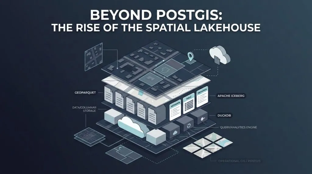
The future is not PostGIS versus the lakehouse. It is a hybrid. PostGIS remains the system of record for live operational GIS, while GeoParquet, Apache Iceberg, and DuckDB support analytical spatial data stored directly on cloud object storage.
This article looks at why traditional analytical GIS workflows are breaking, how the spatial lakehouse stack works, what performance details matter, and where PostGIS still fits in the hybrid GIS future.
Why Analytical GIS Breaks Traditional Workflows
Traditional GIS analytics often begins with a long detour. A new dataset lands in cloud storage. Before anyone can ask a spatial question, the file is downloaded, converted, reprojected, loaded into a database, indexed, queried, and often exported again for another team. The workflow is familiar, but it creates friction at every step.
The first problem is duplication. The original files still exist in cloud storage, while the copied database tables exist somewhere else. This increases storage cost and creates confusion about which version is current. The second problem is slow ETL (Extract, Transform, Load ). Analysts may spend hours preparing data before running the first query. For fast-moving work, that delay matters. The third problem is scaling. A database often couples storage and compute more tightly than a lakehouse-style architecture. As datasets grow, teams may need larger database instances even when the data is only queried occasionally. The final problem is staleness. Once data is exported into local files or side databases, teams can easily end up analyzing old copies instead of the source.
This is where zero-copy data sharing becomes useful. Zero-copy does not mean zero data engineering. It means avoiding unnecessary copying before analysis.
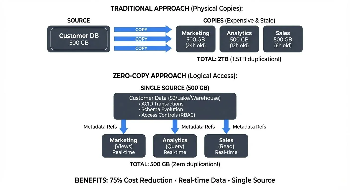
Traditional vs. zero-copy data sharing. Source: Conduktor
In a zero-copy spatial workflow, geospatial data stays in cloud object storage in an optimized format. Multiple tools can then query the same files through governed access, rather than creating new copies for every workflow. DuckDB’s spatial extension and cloud-native geospatial tools show why this is becoming practical: analysts can run spatial SQL closer to the files, without always turning the database into the first stop.
The Three-Part Spatial Lakehouse Stack
A spatial lakehouse is easier to understand if we think of it like a book.
GeoParquet is the pages. It stores geospatial data in the Parquet format, which is column-oriented. Instead of reading every attribute in every row, an analytical engine can read only the columns it needs. If a query only needs geometry and population, it does not have to scan long text descriptions, timestamps, or other unused fields. GeoParquet also adds spatial metadata, so tools can understand geometry columns in a standard way.
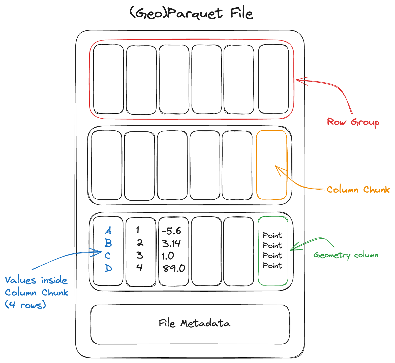
Parquet file layout. Source: Cloud Native Geo
Apache Iceberg is the table of contents. A large spatial dataset may not be one file. It may be thousands of Parquet files spread across cloud object storage. Iceberg organizes those files into reliable analytical tables. It tracks snapshots, schema changes, partitions, and metadata, so different engines can read the same table without losing consistency. This is important when teams need versioned analytical data rather than loose folders of files.
DuckDB is the reader. It is an in-process analytical database that can query files directly using SQL. With the DuckDB Spatial extension, analysts can run spatial operations from a laptop, notebook, or lightweight workflow without maintaining a separate database server. For many exploratory tasks, this makes spatial analytics feel much closer to working with files than managing infrastructure.
In practice, GeoParquet stores the spatial pages efficiently, Iceberg keeps the table organized and versioned, and DuckDB reads the data and runs the queries.
DuckDB has one limitation: scale. DuckDB is excellent for local and embedded analytics, but it is not the only reader. For very large distributed workloads, the same Iceberg tables can also be queried by engines such as Spark, Trino, Snowflake, Databricks, Dremio, or Apache Sedona.
That is the real value of the lakehouse pattern. The data stays in open formats, while different engines can read it depending on the size of the job.
Fast Queries Require Good Layout
A spatial lakehouse is not automatically fast just because the data is stored in the cloud. Cloud storage is cheap and flexible, but it does not know on its own which files are useful for a spatial query.
Imagine a city has millions of building footprints stored across thousands of files. If an analyst asks, “Which buildings are inside this flood zone?”, the system should not open every file in the dataset. It should first identify which files are likely to contain buildings near that flood zone, and ignore the rest.
This is where file layout matters. Iceberg can help by organizing files into partitions, such as country, region, or date. Parquet can store simple statistics about each file or row group. GeoParquet can add spatial metadata, such as bounding boxes, so engines can quickly check whether a file overlaps the query area.
Spatial clustering makes this even better. If nearby features are stored close together, the engine can read less data. Methods such as Z-order and Hilbert curves help arrange spatial data so that nearby locations in the real world are also stored closer together in the file layout. Some platforms also use approaches such as liquid clustering to improve data skipping without depending only on fixed partitions.
Fast lakehouse queries depend on good metadata and good organization. DuckDB, Sedona, Spark, or any other engine can only skip data if the files give them enough information to skip safely. Apache Sedona’s GeoParquet workflow shows how spatial filters can use bounding-box metadata before reading full geometry payloads.
So the lakehouse does not remove data engineering. It changes the work. Instead of spending most of the effort importing files into a database, teams spend more effort organizing files, metadata, and layouts so queries can avoid reading unnecessary data.
The Hybrid GIS Future
The future is not a clean break from PostGIS. It is a better division of labor.
PostGIS remains the operational layer: the place for live editing, spatial constraints, web applications, concurrent users, and transactional safety. The spatial lakehouse becomes the analytical layer: the place for large scans, historical datasets, cloud-native files, and machine learning pipelines. This split is already visible in practice. CARTO is working with major platforms to support Iceberg and GeoParquet as open foundations for cloud-native spatial analytics.
A recent spatial SQL article makes this difference easier to understand using NYC open data. In a spatial join that counted building polygons inside neighborhoods, SedonaDB finished in 0.24 seconds, compared with 6.4 seconds for PostGIS and 43.1 seconds for DuckDB. In a distance query that counted buildings within 200 meters of fire hydrants, SedonaDB took 1.3 seconds, PostGIS took 21.8 seconds, and DuckDB took 41.5 seconds. In a K-nearest-neighbor task that searched for the five closest hydrants to every building, SedonaDB finished in 1.8 seconds, PostGIS took 83.3 seconds, and DuckDB ran into a memory error. The article is worth reading directly because it explains the actual query patterns and practical setup behind the numbers.
These results should not be treated as a universal ranking. They show that analytical spatial workloads behave differently from operational GIS workloads. A live editing system, a national-scale building footprint analysis, and a spatial machine learning pipeline do not need the same architecture.
The real change is not that PostGIS is being replaced. It is that analytical GIS no longer has to begin by importing every dataset into a database. Operational GIS can stay close to PostGIS, while analytical GIS moves closer to open files, cloud storage, and engines built for large scans.
Further Resources

#Deep Tech

Next article
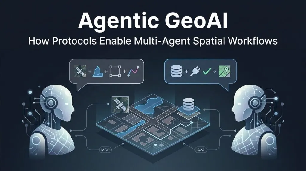
Agentic GeoAI: How Protocols Enable Multi-Agent Spatial Workflows
Ask one AI model to summarize a document, and it may work well. Ask the same model to analyse satellite imagery, query a PostGIS database, compare flood boundaries, calculate road closures, and produce a safe route – the workflow starts to break. Even in narrower tasks such as land-use or land-cover change detection, different ways of comparing satellite embeddings can produce very different maps. The problem here is not intelligence alone – it is context. A GIS workflow usually involves multiple data sources, multiple tools, and many spatial rules for any single model to track all at once.
This is where data misinterpretation becomes dangerous. In a normal chatbot, a wrong answer is frustrating. In a geospatial system, a wrong answer can become a fake road, a missing flood zone, or a route that sends responders into risk. Making the model bigger doesn’t fix this. It is to split the work across specialized agents. One agent handles hydrology, another handles routing, another checks imagery, and another talks to the database. This is the practical next step after Agentic GeoAI: not one general agent, but a coordinated geospatial team.
Two protocols are designed to solve this problem. Anthropic’s Model Context Protocol (MCP) gives an agent a standard way to connect to tools, files, APIs, and databases. Google’s Agent2Agent protocol (A2A) focuses on how agents communicate, delegate tasks, and coordinate across systems. In simple terms, MCP connects an agent to its tools. A2A connects agents to each other.
This article looks at how this “geospatial agent stack” works, why MCP and A2A solve different problems, how a post-disaster routing workflow could be designed, and why geometry data creates new bottlenecks when agents start working together.
Decoupling Collaboration from Capability
To build a reliable map assistant, developers have to separate teamwork from tool use. These are not the same aspects. One layer decides which agent should do the job. The other layer gives that agent access to the right data and tools.
A2A is the horizontal layer. It lets agents discover each other, describe their capabilities, and pass tasks across systems. An emergency response agent does not need to know how a flood analyst agent works internally. It only needs to read its Agent Card, understand what it can do, and send it a task. In GIS, that task might be: “Check whether this road segment intersects the latest flood boundary.”
MCP is the vertical layer. It gives one agent a standard way to use tools. Through MCP tools, an agent can query a spatial database, fetch a STAC item, run a routing function, or call a GIS API. The agent does not need a custom integration for every system. It asks the MCP server what tools exist, then calls the right one.
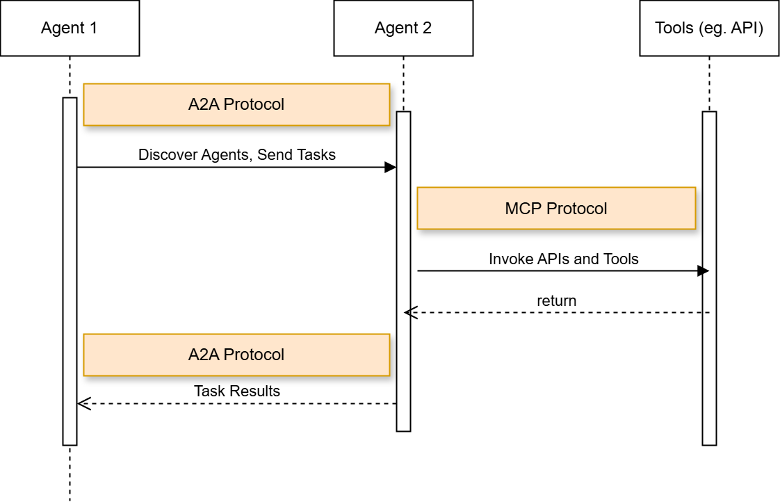
Relationship between A2A and MCP. Source: Gravitee
This split is already appearing in geospatial products. CARTO Agentic Tools let agents create layers, style maps, apply spatial filters, and control deck.gl visualizations. The Felt MCP server connects agents to databases such as Snowflake, BigQuery, Databricks, Postgres, and Redshift. Microsoft’s Planetary Computer Pro MCP tools bring natural-language geospatial workflows into VS Code.
Blueprint in Action: Building a Multi-Agent Spatial Pipeline
A practical version of flood-aware routing already exists. During the 2021 flood disaster in Germany and neighbouring countries, HeiGIT integrated Copernicus EMS flood data into openrouteservice, allowing routes to automatically avoid affected flooded areas. This is a useful real-world example because it connects satellite-derived flood information with routing decisions, which is exactly the kind of workflow disaster response teams need.
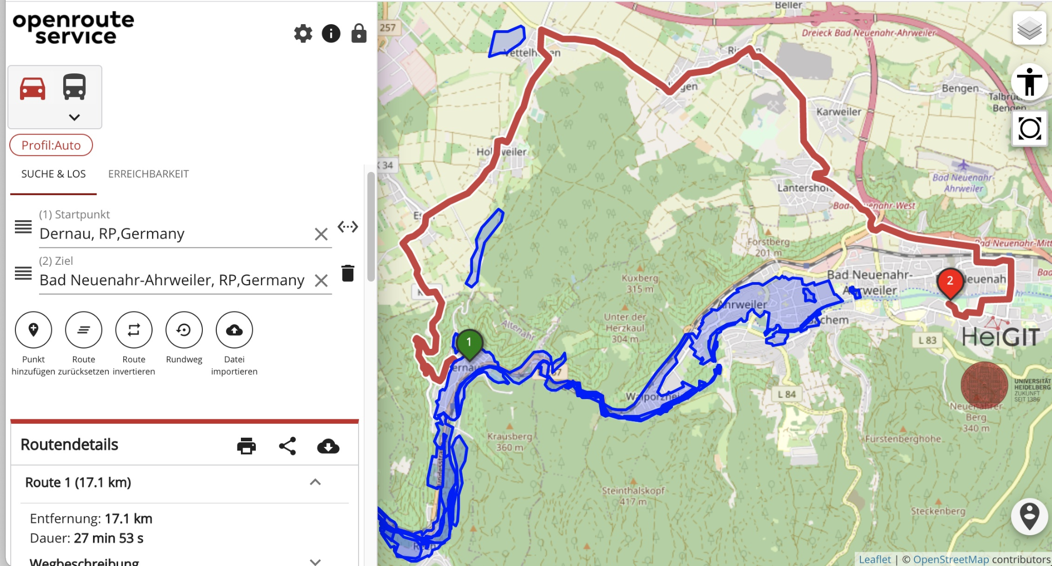
Screenshot of the openrouteservice flood-aware routing tool, showing how Copernicus EMS flood areas can be used to calculate routes that avoid affected zones. Source: HeiGIT
Now imagine building a future agentic version of a similar workflow. Instead of one fixed application handling the entire process, the work could be split across specialized agents. A Coordinator Agent receives the emergency request and defines the area and time window. A Hydro-Analyst Agent evaluates flood extent from recent satellite or SAR imagery. A Geospatial MCP Server provides access to imagery search and water-detection tools. The resulting flood polygon is then passed to a routing service, which avoids flooded roads and generates a safer route. This is where MCP and A2A play different roles. A2A coordinates the handoff between agents, while MCP connects an agent to the tools and data it needs.
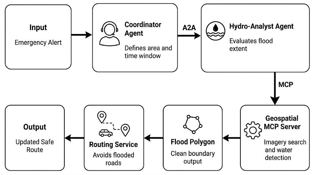
Simplified workflow for an agentic flood-aware routing pipeline
Similar ideas are also appearing in recent disaster-response research. DisasTeller uses multiple vision-language agents for post-disaster assessment, emergency alerts, resource allocation, and recovery planning. ResQConnect presents a human-centred, AI-powered multi-agent platform for flood response planning. These projects do not implement the exact MCP and A2A workflow shown here, but they point toward the same direction: disaster intelligence is becoming more modular, tool-connected, and agent-based.
The Distributed Bottlenecks: State, Tokens, and Geometry Data
Multi-agent GIS does not fail only because agents reason badly. It can also fail because they move the wrong data in the wrong way. A flood boundary, road network, or parcel layer can contain thousands of vertices. If one agent sends a full GeoJSON polygon to another agent as plain text, the system pays for every coordinate as tokens. This creates latency, cost, and context bloat before the model has even started reasoning.
The fix is to pass data by reference, not by value. Instead of sending a 50,000-vertex polygon inside an A2A message, the agent sends a small pointer: an S3 URI, a PostGIS record ID, or a STAC Item. The heavy geometry stays in the data layer. Agents only exchange the reference, then use MCP to fetch, update, or analyze the data when needed.
The efficiency gain: If a raw geometry payload costs P_tokens and the pointer costs R_tokens, then: E = ((P_tokens – R_tokens) / P_tokens) × 100%
For example, replacing a 45,000-token GeoJSON payload with a 25-token URI gives an efficiency gain of about 99.94%. The exact number will vary, but the principle stays the same: do not move heavy geospatial data through prompts.
Source: Medium
This is already how cloud-native geospatial systems work. Cloud Optimized GeoTIFFs allow clients to request only the parts of a raster they need, rather than downloading the whole file. STAC gives those assets searchable metadata and links. In an agentic GIS stack, A2A should carry the intent and the pointer. MCP should handle the actual data operation.
There is also a security benefit. Raw files can contain noise, hidden text, or untrusted metadata. Keeping large payloads in controlled storage reduces what the language model sees directly. Research systems such as Nightjar also point toward a broader pattern: agents should work with shared program state, not endless copies of the same data.
Good geospatial agents know what to carry, and a map reference is almost always enough.
The Protocol-Driven Future of GIS
The next generation of GIS infrastructure will not be defined only by bigger models or closed software suites. It will be defined by open communication layers that let agents, tools, databases, and maps work together without custom integrations for every workflow.
MCP and A2A show how this future can be structured. MCP gives each agent secure access to tools and spatial data. A2A lets agents coordinate with each other across systems. Newer extensions also point to a future where agents could purchase imagery, call paid APIs, or request commercial data under user-approved rules.
The bigger change is already visible in environmental data management. In EnviSmart, a multi-agent workflow processed 2,452 monitoring station datasets and 8,557 published files in two days, while also catching a coordinate transformation error before publication.
For GIS developers, this is the new skill set. It is no longer enough to train a model. The real challenge is learning how to choreograph agents, tools, protocols, and data references into workflows that are fast, secure, and spatially reliable.
Did you like this post? Read more and subscribe to our monthly newsletter!

