#30DayMapChallenge 2024 Highlights from the First 13 Days
#Contributing Writers #Fun

#30DayMapChallenge 2024: Highlights from the First 13 Days

The annual #30DayMapChallenge, created by Topi Tjukanov, is an open invitation to mapmakers of all levels to create and share thematic maps every day in November. Each day presents a new theme, encouraging participants to experiment, learn new tools, and showcase creative takes on classic and contemporary mapping topics. It’s a perfect occasion to express love for all things that are ‘geo’. Here’s a look at the first 13 days and how each theme inspired the community.

Points 📍

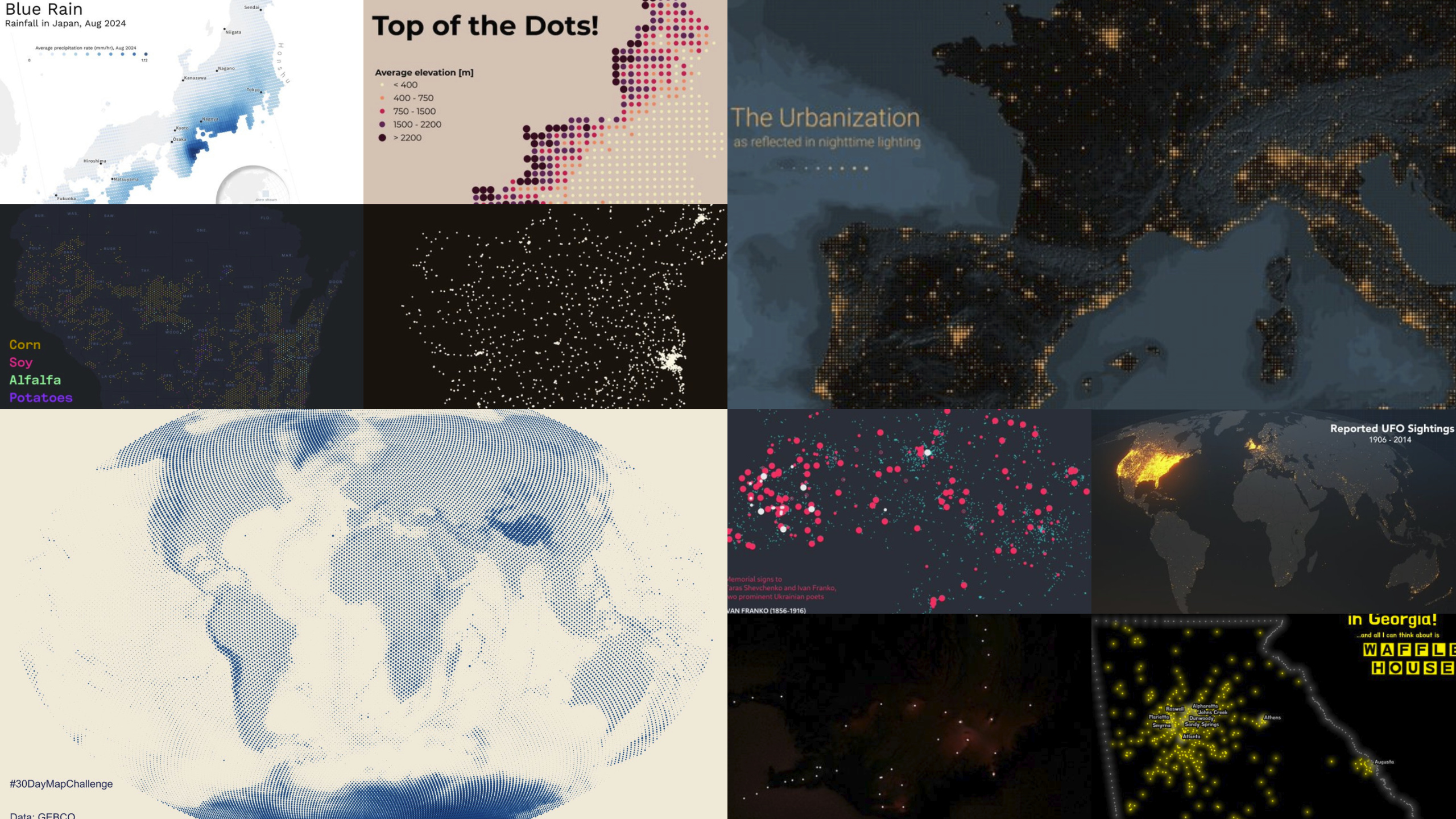
The challenge began with “Points,” focusing on individual locations. From city maps to clusters of natural landmarks, participants used points to represent everything from populations to environmental patterns, underscoring the foundational role of points in mapping.
#30DayMapChallenge 2024 - points

Lines 📏

“Lines” invited mappers to capture connections and boundaries through roads, rivers, and flight paths. This theme emphasized the beauty of linear features, showing the world’s movement and divisions.
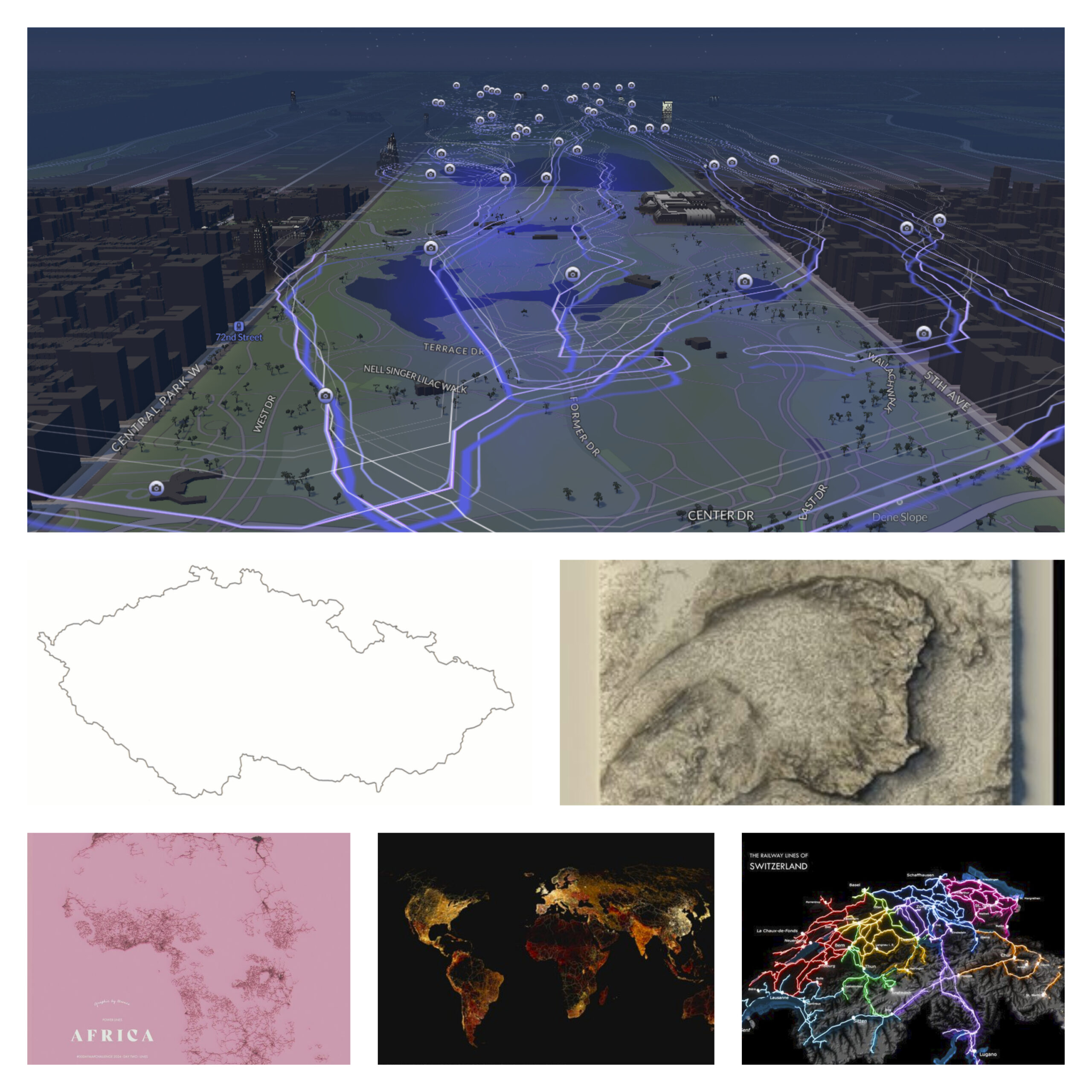
#30DayMapChallenge 2024 - lines

Polygons 🛑

Polygons added depth, allowing participants to visualize defined regions and areas, from city zones to climate regions. This theme highlighted the diversity of areas that can be mapped using filled shapes.
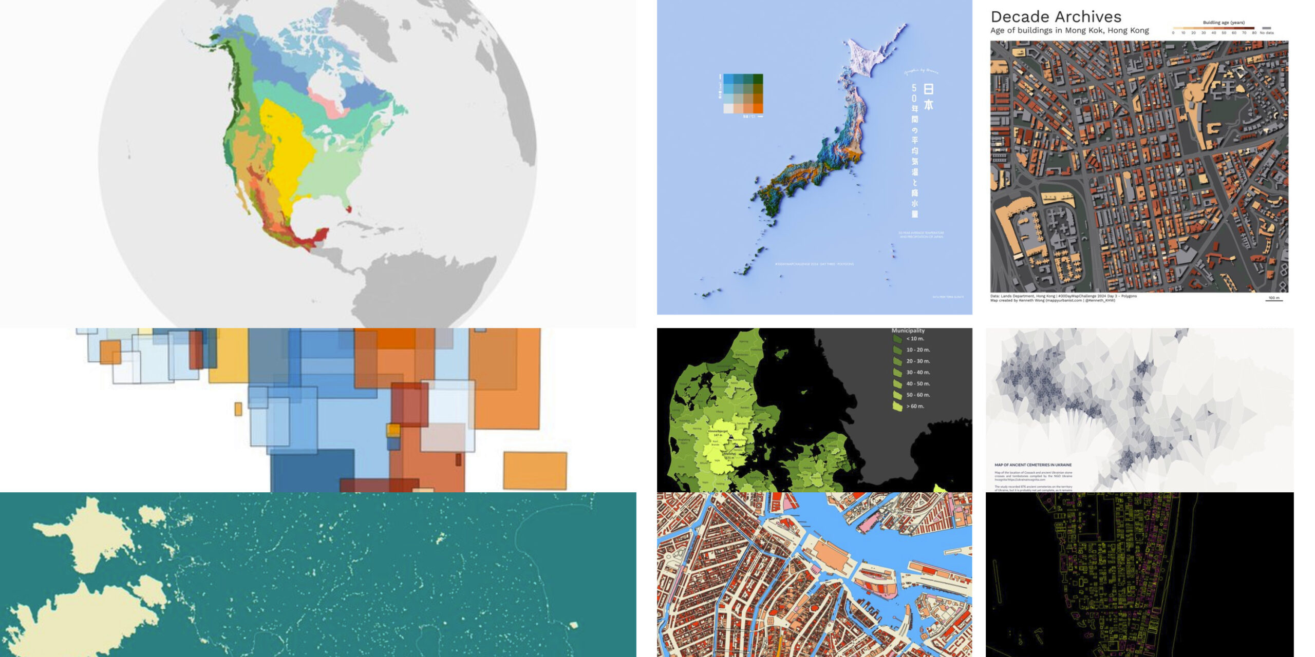
#30DayMapChallenge 2024 - polygons

Hexagons 🔷

Swapping square grids for hexagons, participants created smoother visual representations of density, movement, and spatial patterns. Hexagonal grids were popular for visualizing urban layouts and distribution patterns.
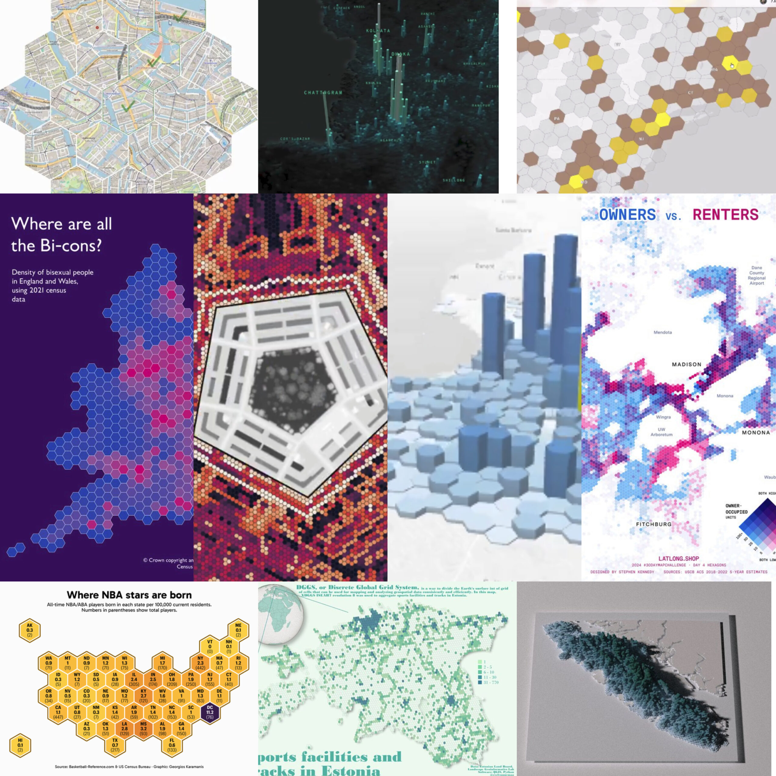
#30DayMapChallenge 2024 - hexagons

A Journey 🚶‍♂️✈️

“A Journey” brought narrative into maps, encouraging participants to trace paths, from personal commutes to historical explorations. Each map represented a unique story of movement across places and time.
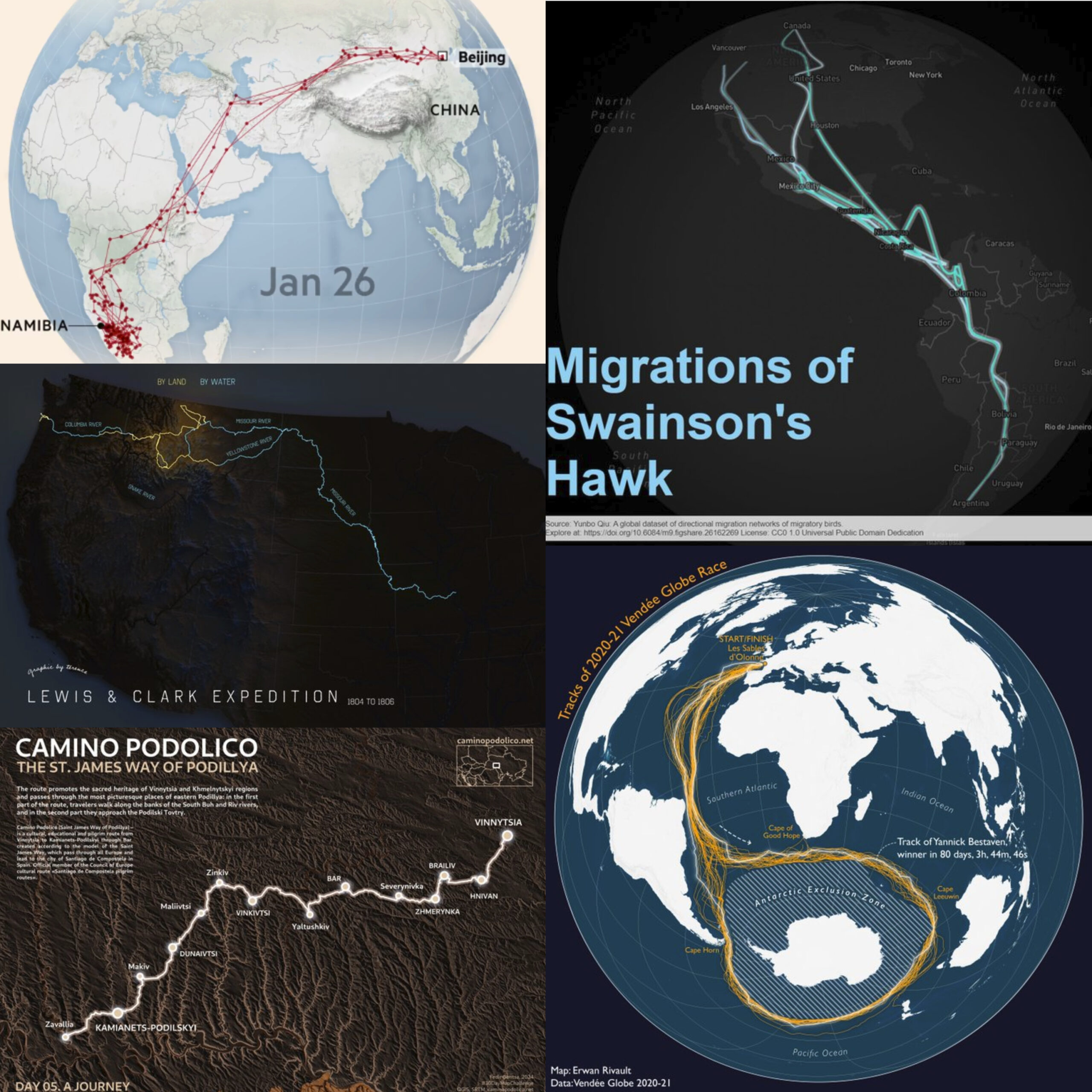
#30DayMapChallenge 2024 - a journey

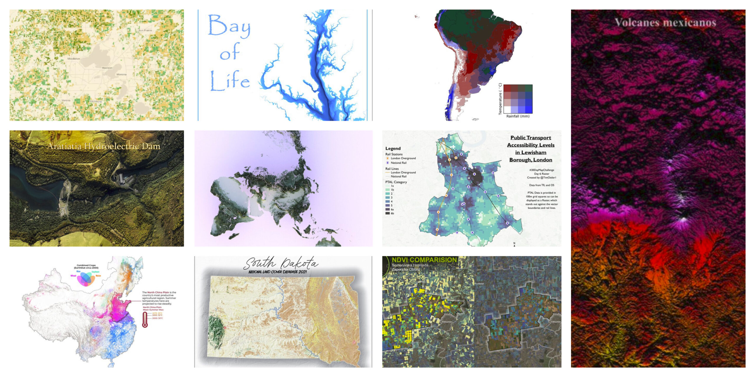
Raster 🟦🟧

Using raster data, mappers highlighted the continuous surfaces found in satellite imagery, heatmaps, and population density maps. The results showed the flexibility of pixels in visualizing everything from temperature shifts to nighttime city lights.
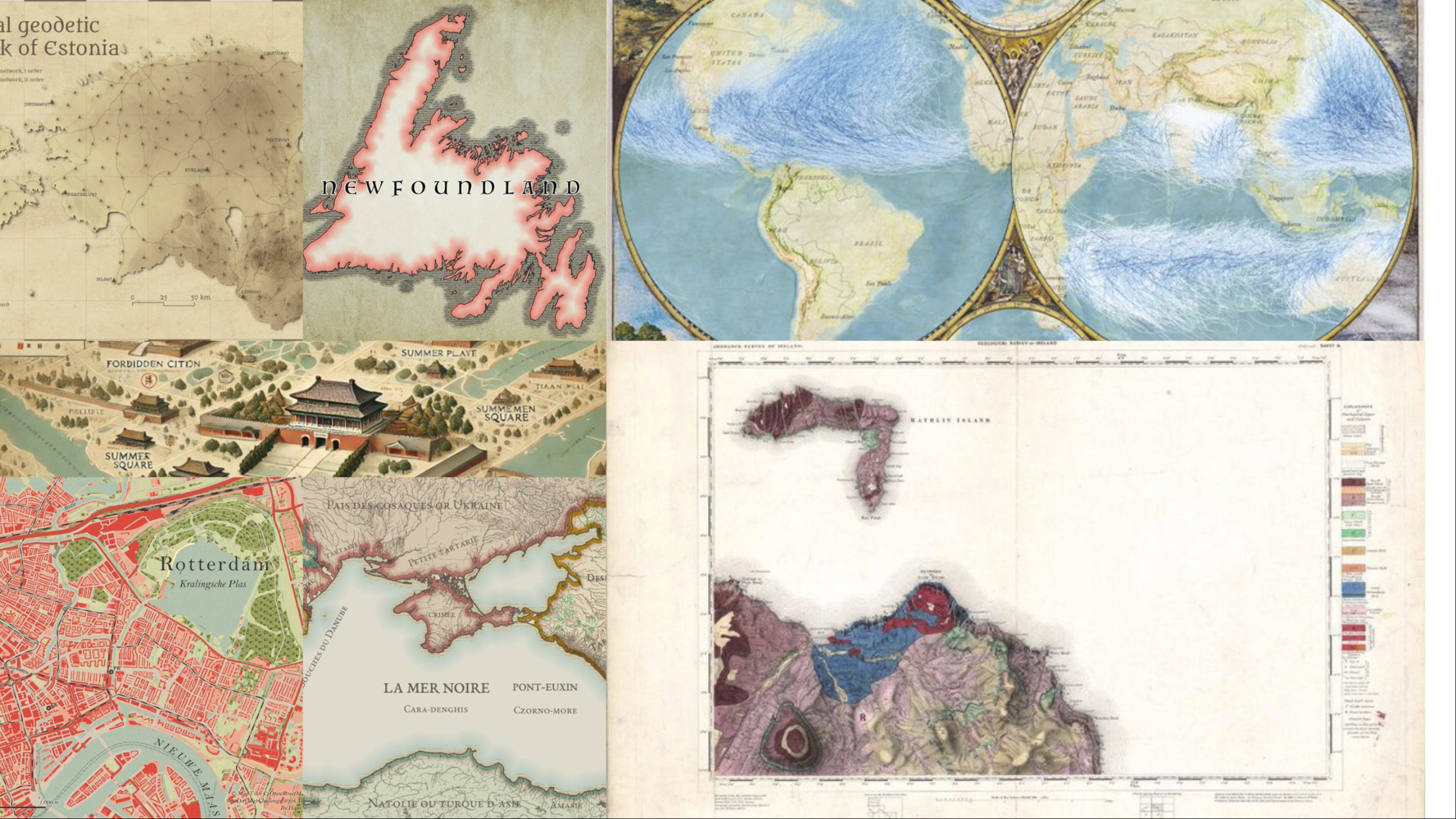
Vintage Style 🕰️🗺️

This theme let mappers add a nostalgic twist, using vintage aesthetics for modern subjects. The maps captured an old-world charm with muted colors and antique fonts while addressing contemporary topics.
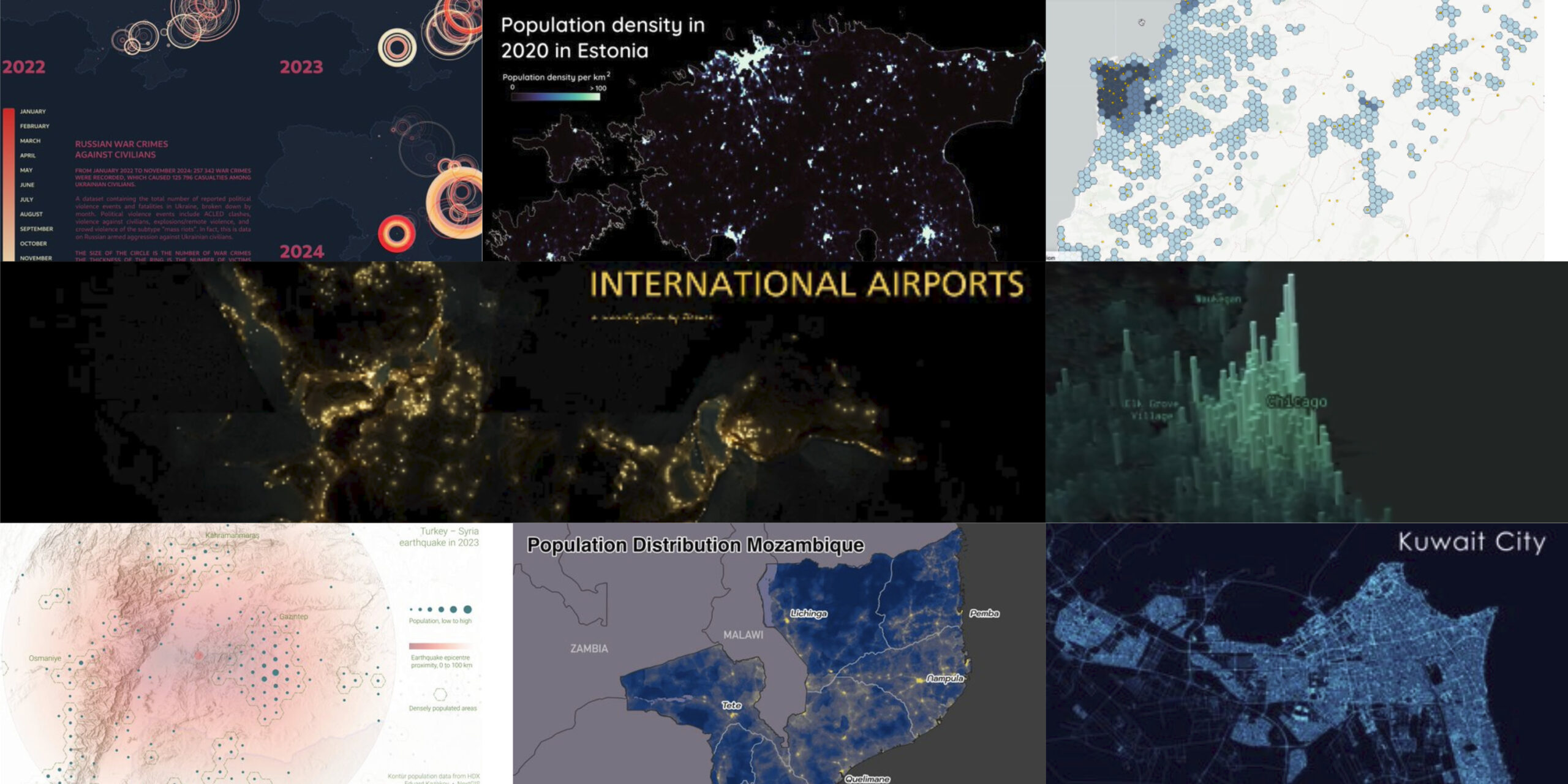
Humanitarian Data Exchange (HDX) 🌍🚑

“HDX” focused on humanitarian mapping, using data from the Humanitarian Data Exchange to address issues like health, disaster response, and development. The maps brought attention to vulnerable areas, reminding us of data’s role in social impact.
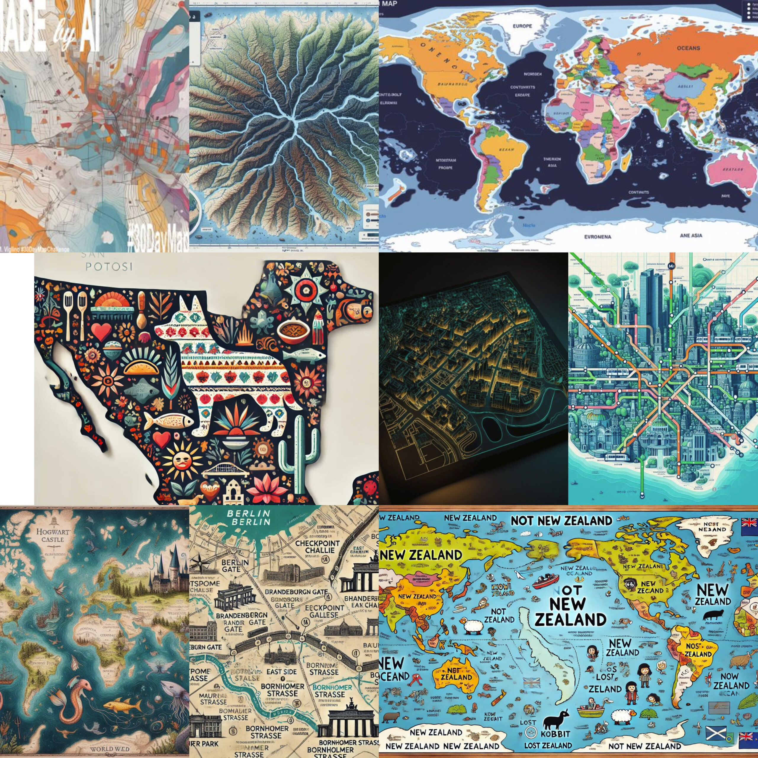
AI Only 🤖

On this day, participants experimented with AI tools like DALL-E and ChatGPT, using prompts to generate maps. This exercise pushed the boundaries of AI’s potential in cartography, sparking discussions on its limitations and strengths.
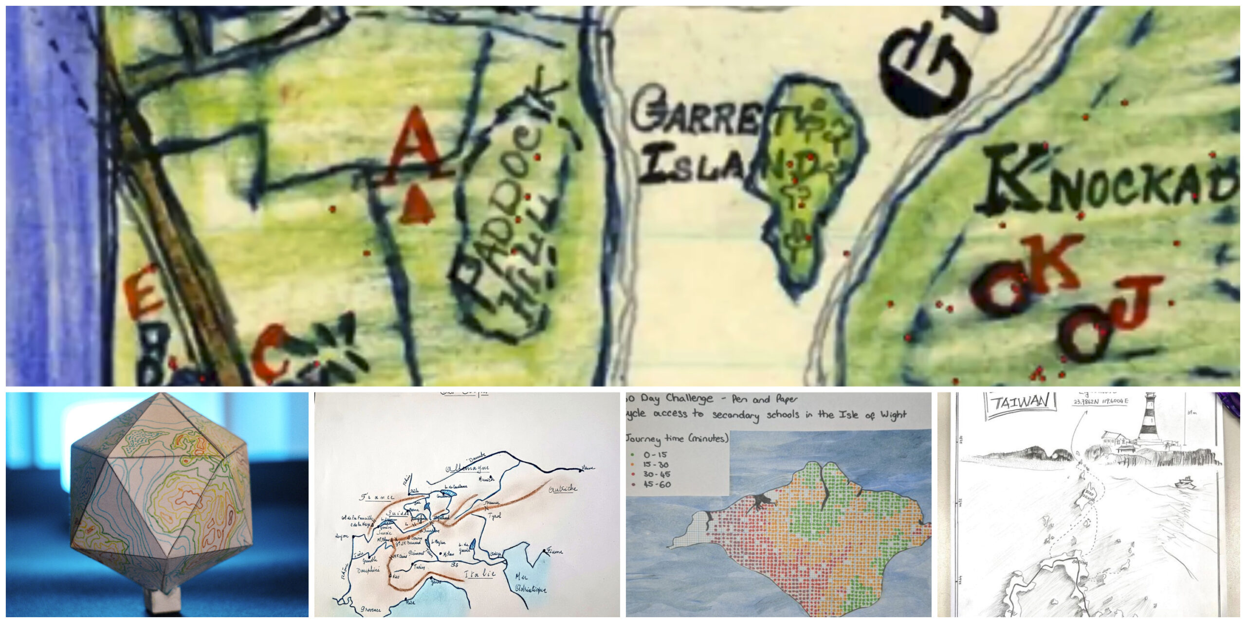
Pen & Paper ✏️🗺️

“Pen & Paper” day invited participants to step away from screens and draw by hand, highlighting the personal and artistic side of mapmaking. From simple sketches to detailed fantasies, each map was a unique piece of analog creativity.
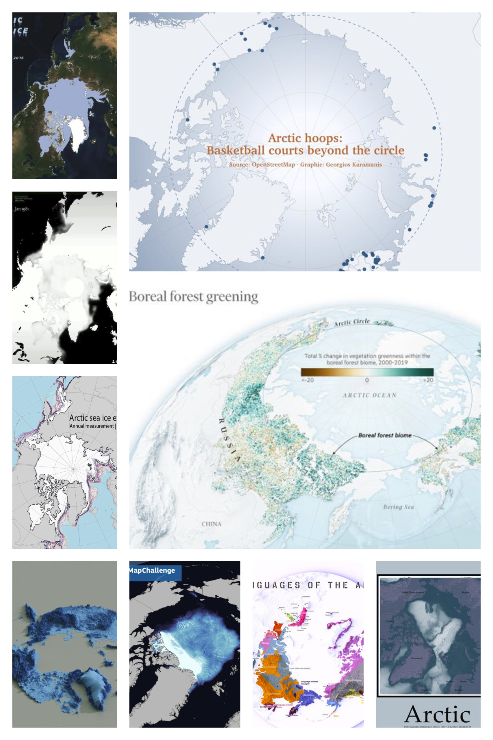
Arctic ❄️🧊

Maps of the Arctic emphasized critical topics like ice coverage, wildlife habitats, and climate change effects, reminding viewers of the urgent environmental issues affecting polar regions.
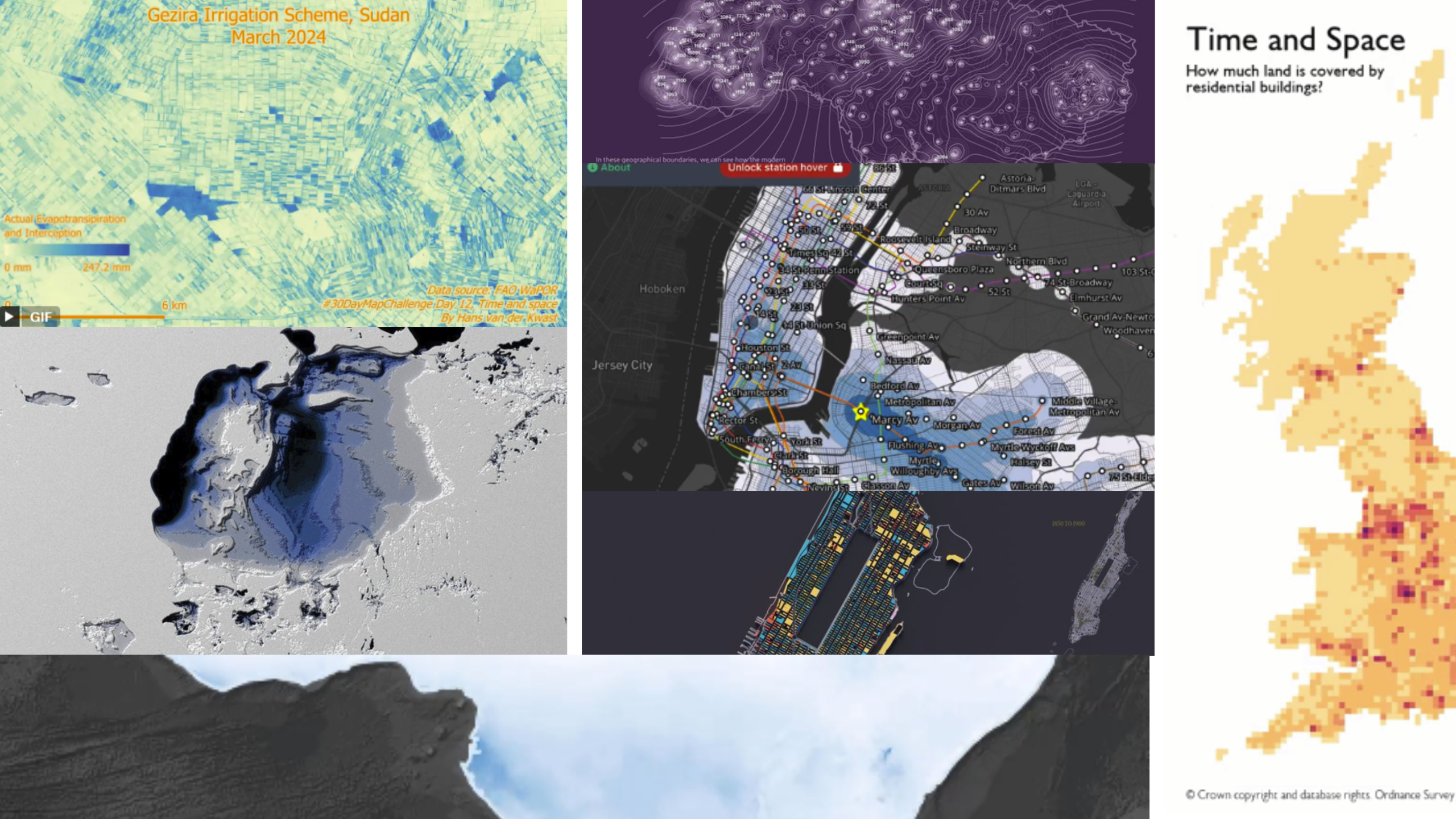
Time and Space ⏳🌍

Mapping time allowed participants to show change over periods, from urban expansion to wildlife migration. This theme highlighted the relationship between geography and time, bringing dynamics into spatial data.
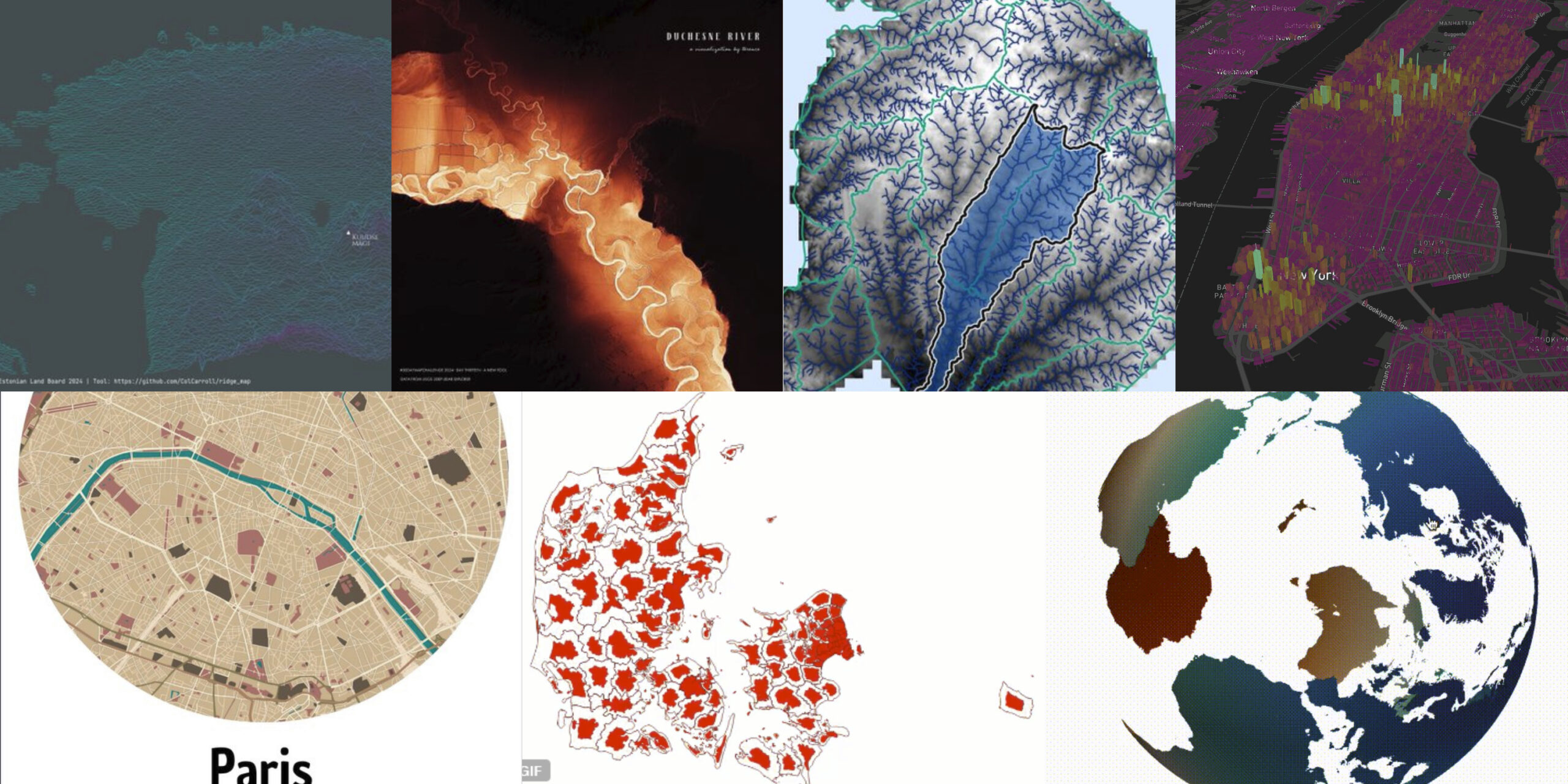
A New Tool 🧪🔧

On the thirteenth day, participants tried out new tools or techniques, staying true to the challenge’s spirit of experimentation. From 3D visualizations to artistic interpretations, this day showcased the thrill of learning something new.
These first 13 themes of the #30DayMapChallenge illustrate the range and creativity in the cartography community. The challenge continues, promising even more inspiring contributions as mappers try to map the remaining topics.


Sources

  • Points

https://x.com/fede_gaspari/status/1852251732086018157

https://x.com/oh_sk/status/1852264030984880484

https://x.com/nextgis/status/1852250773809230230

https://x.com/geo_alyaqout/status/1852387513609892150

https://x.com/Kenneth_KHW/status/1852300883142549890

https://x.com/ceren_do/status/1852404159741600252

https://x.com/researchremora/status/1852529323367907540

https://x.com/gontsa/status/1852449613665411450

https://x.com/XenonGT/status/1852384564401811629

https://x.com/jrncarlock/status/1855014892266262771

  • Lines

https://x.com/Julian_H0ffmann/status/1853739665917907307

https://x.com/PythonMaps/status/1853493302995161436

https://x.com/Mapbox/status/1852742670633906680

https://x.com/skopmichal/status/1852838481292116360

https://x.com/fede_gaspari/status/1853389649030402151

https://x.com/BhuvanamitraS/status/1852700162671415522

https://x.com/researchremora/status/1852688224415608957

  • Polygons

https://x.com/kyle_e_walker/status/1853089761814327487

https://x.com/IvaBrunec/status/1853232363121053723

https://x.com/ErwanRivault/status/1853062183040569682

https://x.com/evelynuuemaa/status/1852998339869986912

https://x.com/researchremora/status/1853052728320123216

https://x.com/Kenneth_KHW/status/1853069909649195238

https://x.com/geomenke/status/1853025391620862369

https://x.com/gontsa/status/1853205196232380436

https://x.com/tjukanov/status/1852969630307877074

https://x.com/MashfordMahute/status/1853089602988355773

https://x.com/jbrichman/status/1853114809291583834

  • Hexagons

https://x.com/OrdnanceSurvey/status/1853470336240558239

https://x.com/Mapbox/status/1853482649068720315

https://x.com/felt/status/1853489932331106551

https://x.com/mapchannels/status/1853252649451172222

https://x.com/JackSapoch/status/1853508208045818367

https://x.com/kyle_e_walker/status/1853452143971434698

https://x.com/geokaramanis/status/1853469941833331132

https://x.com/oh_sk/status/1853408025270186140

https://x.com/evelynuuemaa/status/1853363807998902552

https://x.com/IvaBrunec/status/1853589870612021437

  • A journey

https://x.com/sdbernard/status/1854230197714690497

https://x.com/ErwanRivault/status/1853780808781140465

https://x.com/gontsa/status/1853953677683466719

https://x.com/eye_am_the_i/status/1853847795909714159

https://x.com/researchremora/status/1853925623183380674

  • Raster

https://x.com/oh_sk/status/1854136763809141176

https://x.com/SouthCrossMaps/status/1855404253235581181

https://x.com/GWSCatUA/status/1854276614558802062

https://x.com/MapsChartsData/status/1856195295136096735

https://x.com/researchremora/status/1854223275884175649

https://x.com/XenonGT/status/1854216790949105712

https://x.com/PythonMaps/status/1854931890748240190

https://x.com/TimOstler1/status/1854097705049391223

https://x.com/AlcisGeo/status/1854205856713236636

https://x.com/JosArturoJasso/status/1854402013175455867

  • Vintage style

https://x.com/evelynuuemaa/status/1854443646554132520

https://x.com/MapsChartsData/status/1856196104921944345

https://x.com/c_yatteau/status/1856373524128026731

https://x.com/jacobmac02/status/1855977905458675932

https://x.com/hansakwast/status/1854425001270653185

https://x.com/gontsa/status/1854650482066870291

https://x.com/GeoSurveyNI/status/1854432662380843203

https://x.com/TheYuanLiao/status/1855188041318461721

  • Data: HDX

https://x.com/geodatascience/status/1854856399471165518

https://x.com/researchremora/status/1854864795649933497

https://x.com/gontsa/status/1855063834387513806

https://x.com/oh_sk/status/1854852346422911285

https://x.com/jacobmac02/status/1855979732497473845

https://x.com/evelynuuemaa/status/1854807823156494401

https://x.com/geo_alyaqout/status/1854915271758123408

https://x.com/nextgis/status/1854785401648472142

  • AI only

https://x.com/jmviglino/status/1855145842178449430

https://x.com/Mapologies_com/status/1855185175421874244

https://x.com/evelynuuemaa/status/1855250324086235466

https://x.com/athnfrnclr/status/1856439926620836058

https://x.com/mildthing99/status/1855037220677124518

https://x.com/hansakwast/status/1855186588986184155

https://x.com/AlcisGeo/status/1855293020112925079

https://x.com/OrdnanceSurvey/status/1855218952525251033

https://x.com/GastonEchenique/status/1855454120489951296

https://x.com/renorosgon/status/1855645758252290194

https://x.com/MaiGhalyGazzar/status/1855290002432790536

https://x.com/undertheraedar/status/1855196452009464241

  • Pen & paper

https://x.com/AlandcoC/status/1855546846359286079

https://x.com/nextgis/status/1855562886631887080

https://x.com/mildthing99/status/1855408669636116598

https://x.com/basemap/status/1855566069978542528

https://x.com/jjakon11/status/1855754593889927215

  • Artctic

https://x.com/geokaramanis/status/1855954998925897886

https://x.com/hansakwast/status/1855859502442008661

https://x.com/sdbernard/status/1856275572235587766

https://x.com/PythonMaps/status/1856446245054681520

https://x.com/eye_am_the_i/status/1856448896777498656

https://x.com/kai_sonder/status/1855989027951833198

https://x.com/CMEMS_EU/status/1855890712467751411

https://x.com/researchremora/status/1856025139655086347

https://x.com/jjakon11/status/1856159442498400604

  • Time and space

https://x.com/gontsa/status/1856474790825017775

https://x.com/IvaBrunec/status/1856337606297952313

https://x.com/Mapbox/status/1856381452843393340

https://x.com/OrdnanceSurvey/status/1856376315110133923

https://x.com/researchremora/status/1856350965915426948

https://x.com/nextgis/status/1856241145224802471

https://x.com/hansakwast/status/1856246957691257118

  • A new tool

https://x.com/maaamet/status/1856651606374203459

https://x.com/researchremora/status/1856797227504865742

https://x.com/GeoWithJustin/status/1856789887569059955

https://x.com/IvaBrunec/status/1856709487563813077

https://x.com/laMartu30/status/1856653972460757405

https://x.com/geomenke/status/1856725882531979675

https://x.com/joseph_barbier/status/1856609596430860572


How do you like #30DayMapChallenge initiative? Read more and subscribe to our monthly newsletter!

Say thanks for this article (1)
The community is supported by:
Become a sponsor
#Contributing Writers
#Fun
Fictional Maps: Crafting Online Fantasy Worlds
Sebastian Walczak 06.21.2024
AWESOME 1
#Fun #Ideas #People
‘You Are #Geoawesome’ Original Series: A Step-by-Step Guide
Sebastian Walczak 10.9.2024
AWESOME 0
#Contributing Writers #Fun #Satellites #Science
An Overview of Indices in Remote Sensing
Sebastian Walczak & Nikita Marwaha Kraetzig 07.3.2024
AWESOME 1
Next article
#Featured #Science

A Global Road Surface Type Classification Dataset Powered By Deep Learning and Mapillary Data

The Importance of Surface Data Drives Transportation, Safety, and Economic Development

Road surface information plays a crucial role in various sectors, from transportation safety to economic growth and environmental sustainability. Accurate road surface data informs decisions around route planning, driving conditions, and emergency response logistics. 

For instance, unpaved roads, especially in wet or poorly maintained conditions, pose increased risks of accidents, while knowledge of road types (paved vs. unpaved) aids in selecting appropriate routes for ambulances, fire trucks, or other emergency services in areas with limited infrastructure.

This data also optimizes supply chains, agricultural infrastructure, and logistics, reducing transportation costs and delays. For tech applications like Open Street Map (OSM), and GPS systems, reliable road surface data improves routing, especially in rural and underdeveloped regions, enhancing navigation and route selection for drivers.

Beyond Building Footprints: Enriching OSM Attributes

Enriching OpenStreetMap (OSM) with detailed attributes is essential for maximizing its value as a tool for decision-making and efficient service delivery. While OSM provides an impressive level of global road coverage—estimated at about 83%—significant gaps remain in critical metadata, such as road surface types. Only 30-40% of roads in the dataset have surface type information, and this deficiency is even more pronounced in developing regions.

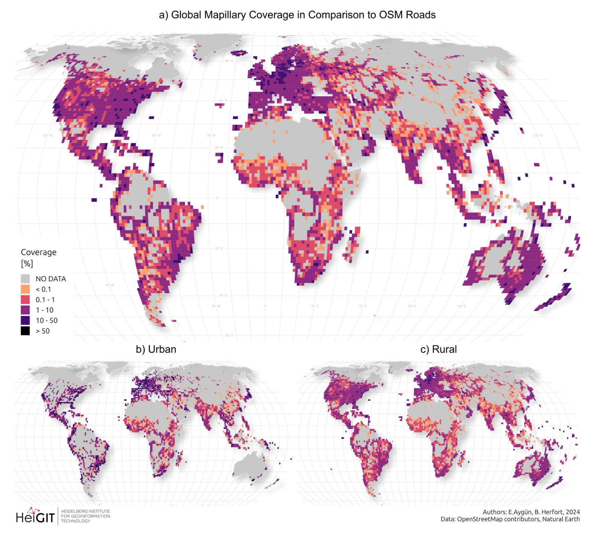
Global overview of spatial distribution of OpenStreetMap (OSM) road length coverage derived from Mapillary data (based on zoom 8 tiles). The maps illustrate: (a) Total OSM Road Length Coverage, (b) Urban OSM Road Length Coverage, and (c) Rural OSM road Length Coverage, showing the varying degrees of coverage across different regions of the world. The color gradient from blue to yellow indicates the percentage of length coverage, with lighter colors representing higher coverage.

To address this, we at HeiGIT (Heidelberg Institute for Geoinformation Technology), are releasing a global dataset on road surface types (paved or unpaved), contributing to humanitarian response, urban planning, and economic development goals. By making this information openly available, we aim to enrich global mapping efforts, especially in regions lacking detailed infrastructure data. 

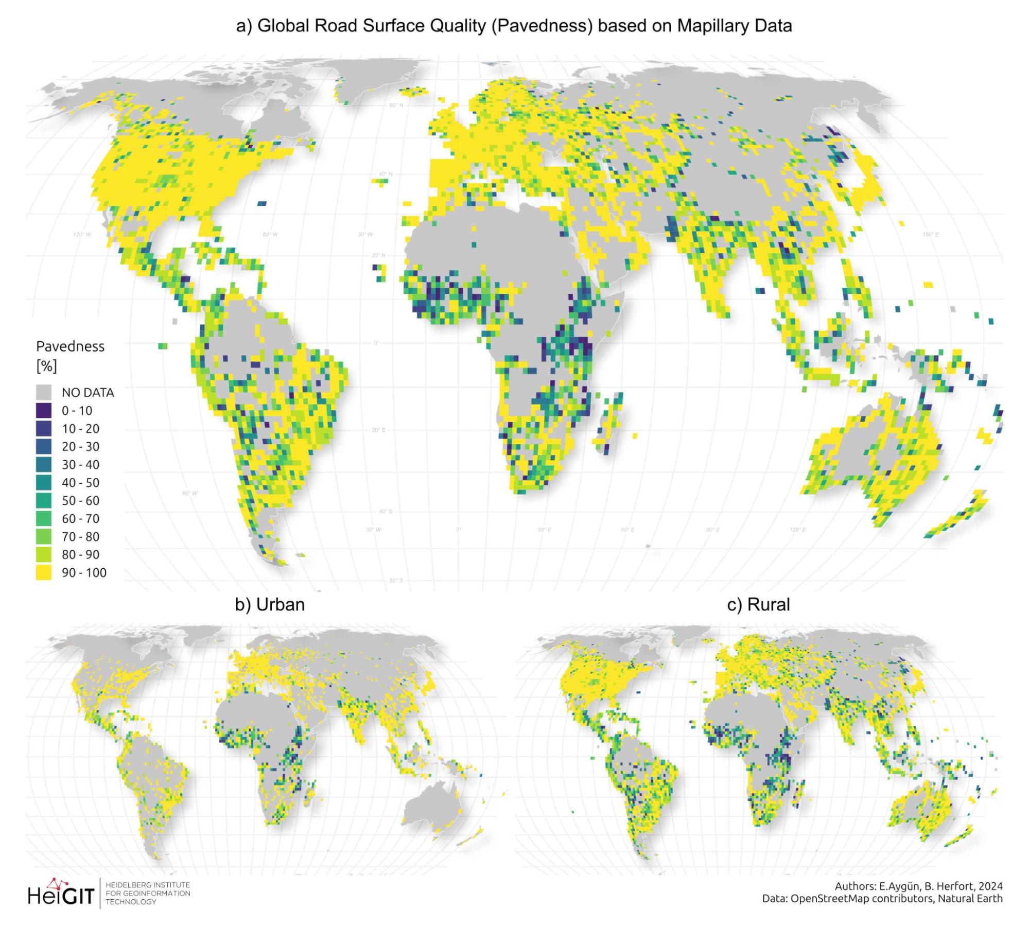
Distribution of road surface quality predicted based on Mapillary data: (a) total pavedness (defined as the ratio of total paved roads w.r.t total OSM roads for each zoom 8 tile), (b) and (c) pavedness per tile, calculated for urban and rural areas respectively.

How We’re Using Deep Learning to Classify Road Surfaces

At HeiGIT, we’ve made significant strides in improving global road surface classification using cutting-edge deep learning techniques. A major challenge is the diversity of road imagery, especially from crowdsourced platforms like Mapillary, which provides vast street-view images worldwide. To address this, we deployed a SWIN-Transformer model pre-trained on the ImageNet-1k dataset and fine-tuned it on our own street-view imagery, creating a planet-scale application that sets new benchmarks for road surface classification accuracy.

Why the SWIN-Transformer?

We chose the SWIN-Transformer (Shifted Window Transformer) architecture because of its proven ability to establish long-range dependencies, making it highly effective at extracting global features from images. This model excels with heterogeneous data, like street-view imagery from various regions, as it captures fine-grained details crucial for road surface classification. Its ability to analyze the surrounding context enhances classification accuracy.

Crowdsourced Data and Training

The training dataset for our model came from an event at Heidelberg University in July 2023, where 30 volunteers participated in a mapathon using the HeiGIT CrowdMap web application. These volunteers labeled 20,000 random Mapillary images from 39 countries in sub-Saharan Africa, classifying them as “paved,” “unpaved,” or “bad imagery.” This labeling process played a critical role in building a reliable training set for the model.

Once the data was collected, we split the dataset into training and validation sets. After training, our model achieved a validation accuracy of 98.5%. To optimize the model’s performance, images in the training set were cropped from their original size of 2000×1200 pixels to 427×256 pixels, improving time and space complexity without sacrificing classification accuracy. To enhance the model’s robustness, we used data augmentation techniques, increasing the diversity of the images and improving the model’s generalization capabilities.

Tackling Anomalous Images with Advanced Filtering

One of the challenges we encountered during this process was the presence of anomalous images that didn’t contain any roads, such as images featuring sidewalks, side views, or tracks. These images, though unrelated to the task at hand, were being classified with respect to road surface information, which introduced noise into the dataset.

To address this, we implemented a combination filter using two additional models:

  1. A Fast Semantic Segmentation Model: Based on the PIDNet architecture, pre-trained on the Cityscapes dataset, this model was used to filter out images where road pixels comprised less than 10% of the total pixels. This ensured that only images containing substantial road views were considered for classification.
  2. CLIP Model for Zero-Shot Classification: We also incorporated CLIP (Contrastive Language–Image Pre-training), a zero-shot classification model based on the ViT-L/14 Transformer architecture. This model helped identify images with no roads by using two predefined classes: “a photo of a road” and “a photo with no road in it.” If the model predicted an image to be “a photo with no road in it” with a probability score of greater than 90%, it was filtered out.

The final filtering process removed images where the road pixel coverage was less than 10%, or where the CLIP model confidently predicted the absence of roads. This filtering stage eliminated approximately 4-5% of the total images, ensuring that our model only analyzed relevant data.

Performance and Validation: How Well Does It Work? 

Once trained, the SWIN-Transformer model was validated against OpenStreetMap (OSM) surface data using a total of 5.16 million images from around the world. 

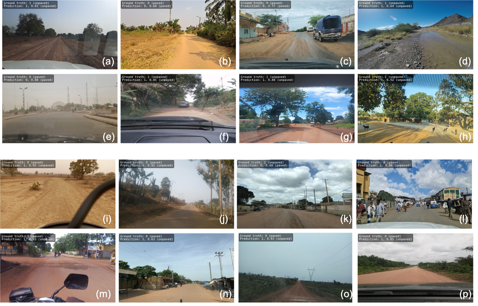
The results were impressive, with F1 scores ranging from 91% to 97% for paved roads across different continents. However, there was some overestimation for the prediction of unpaved roads which was largely impacted due to the heterogeneous quality of Mapillary 

Images lacked clear, direct frontal views of roads and instead consisted of side views of houses, driveways, and landscapes. This validation confirmed the model’s robustness and reliability in classifying the majority of road surfaces accurately on a global scale.

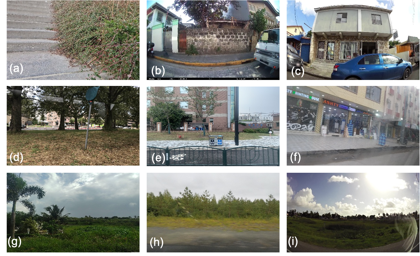
The figure above shows examples of predictions for the SWIN Transformer. Ground Truth, Prediction, and confidence score are indicated in the top left corner of each image. 

The figure above shows examples of poor-quality images from Mapillary that contributed to false negative predictions in the SWIN Transformer model.

Big Data for Download, Processing, and Analytics: A Scalable Approach

At HeiGIT, we’ve leveraged tools like DuckDB and Apache Parquet to streamline data processing and enhance our deep learning pipelines.

DuckDB for High-Performance Analytics

For processing large datasets, we relied on DuckDB, an open-source SQL database management system designed for high-performance analytical queries. DuckDB excels at efficiently managing big data, allowing us to run complex queries while minimizing processing time and resource consumption.

Apache Parquet for Efficient Data Storage

To optimize data storage and retrieval, we employed Apache Parquet, an open-source, column-oriented file format that compresses data for efficient bulk processing. Parquet allows us to handle complex datasets while ensuring that both storage and retrieval processes are fast and scalable.

Downloading Global Mapillary Data

The Mapillary API provides two primary methods of accessing data: vector tiles and entity endpoints. We utilized both to download street-view images from across the globe. 

The process started with creating a zoom level 8 (z = 8) map of the world, filtering out ocean areas using continent polygons. From this, we extracted tiles that contained Mapillary sequences. We downloaded a staggering 11,031,802 sequences using the tiles endpoint, where each sequence represents a series of GPS nodes linked to images. These sequences were then processed using the entity endpoint to retrieve detailed image metadata, resulting in over 2.2 billion metadata points. This enormous dataset provides the foundation for various machine learning and deep learning applications.

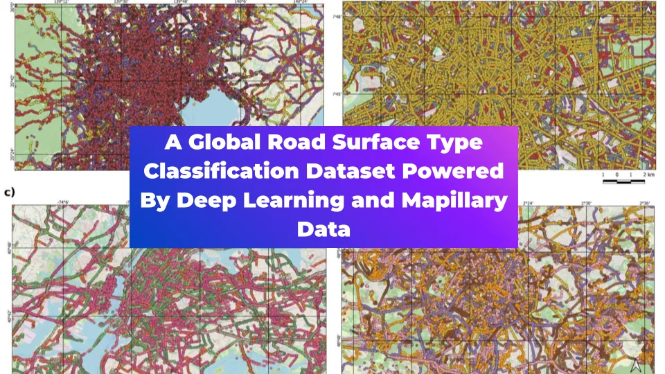
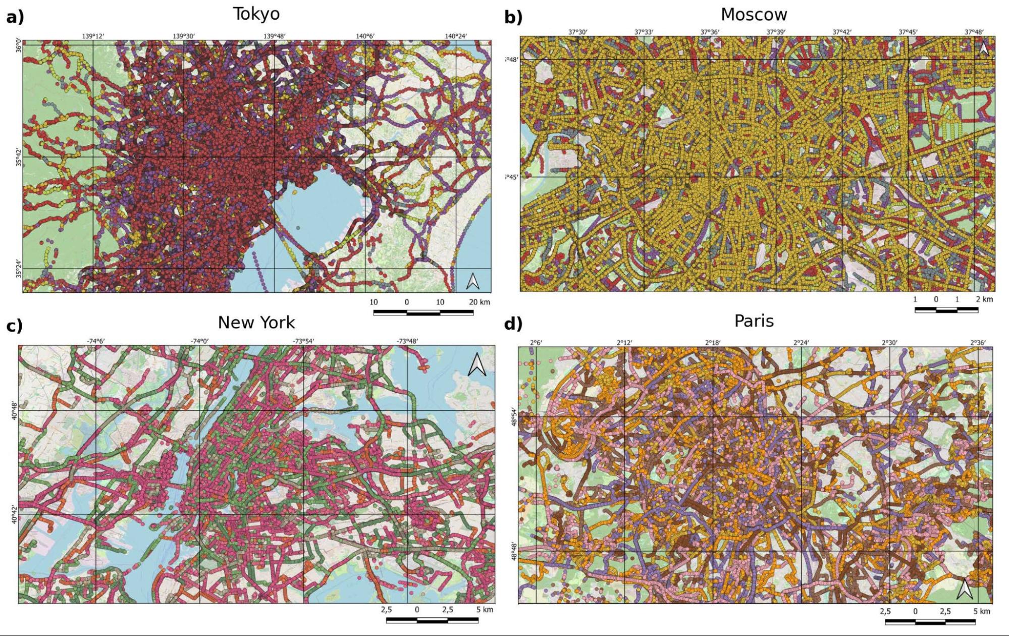
Map visualizations of road sequence data from various global urban areas. Each panel displays sequences that have been color-coded where possible, although the high volume of sequences in areas such as Tokyo and Moscow prevents distinct color coding. The different colors observed in sequences from San Francisco and Paris indicate various sequences; however, due to the limited color palette, a single color may represent multiple sequences.

Spatial Filtering for Relevant Images

Given the vast dataset, we performed spatial filtering to focus on the most relevant images for our road classification tasks. A spatial gap of 1000m for non-urban areas and 100m for urban areas was used to reduce redundancy. Urban centers were identified using two datasets:

  • Africapolis for Africa.
  • Global Human Settlement Layer Urban Centres Database (GHS-UCBD) for other parts of the world.

Map Matching with OSM Data

Mapillary images offer a rich potential for adding valuable attribute information to OpenStreetMap (OSM) features without needing extensive field surveys. However, due to slight inaccuracies in the geo-referencing of both datasets, we had to employ map matching techniques. Using the ohsome API, we extracted relevant OSM road objects filtered by the ‘highway’ tag based on their spatial location.

Map matching was conducted by calculating the shortest Euclidean distance between the centroid of Mapillary images and nearby OSM road segments. Images within 10 meters of an OSM road segment were directly assigned to that segment, accounting for typical GPS errors of up to 5 meters. For images farther away, additional thresholds of 20 meters and 30 meters were applied in subsequent steps.

A Confidence Index for Map Matching Accuracy

To standardize the assignment of image points to OSM segments, we developed a normalized confidence index. This index captures the contrast in distance between the nearest OSM segment and surrounding segments within a defined boundary box. The index helps ensure that each image point is confidently assigned to the most relevant OSM road segment, improving the accuracy of our spatial data processing.

Our scalable approach to big data processing, using state-of-the-art tools like DuckDB, Apache Parquet, and the Mapillary API, allows us to process and analyze vast amounts of street-view imagery efficiently. By combining these techniques with advanced map matching methods and spatial filtering, we ensure that our datasets are optimized for downstream applications like geospatial analysis.

For readers interested in deeper data insights, our latest analysis of the final dataset, available in the preprint, reveals intriguing global trends in road surfaces and Mapillary coverage, highlighting patterns in both urban and rural infrastructure.

Conclusion

As road infrastructure remains a critical metric for socio-economic development, our global road surface dataset will offer valuable insights for a wide range of applications, helping to build a more connected and resilient world.

Our road surface classification model represents a significant leap forward in global mapping and geospatial analysis. By leveraging advanced deep learning techniques, big data analytics, and crowd-sourced data, we’ve developed a model that can accurately classify roads as paved or unpaved across diverse regions and conditions. This work not only contributes to better mapping tools but also has practical applications in transportation planning, infrastructure development, and humanitarian response efforts. Routing services that cater to diverse mobility needs, such as those designed for emergency services or freight transport, benefit significantly from enriched surface type data.

The dataset generated and analyzed is openly available at the The Humanitarian Data Exchange and as a scientific preprint. If you’re interested in learning more about the data insights, check out HeiGIT’s latest blog post. We have enriched the dataset with a set of attributes with relevant Mapillary as well OSM segment information (corresponding to the OSM road segment matched to the Mapillary image point) for each image point, thereby facilitating further usage of this dataset for a variety of downstream analyses in a context of geospatial applications or then computer vision modeling benchmarking efforts.


For more details on this work, please refer to the preprint available on arXiv at http://arxiv.org/abs/2410.19874 

Read on
Search