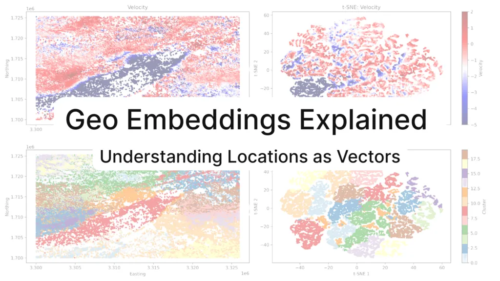
Geo Embeddings Explained: Understanding Locations as Vectors

In geospatial analysis, a basic but often implicit challenge is enabling a computer to reason about distance – for example, to recognize that Munich is closer to Augsburg than to Tokyo.
If we give a machine learning model raw latitude and longitude, it often fails to understand distance correctly. Most models treat numbers as if they lie on a flat grid. They assume a simple x and y space. But the Earth is round, not flat. Because of this, a one-degree change in longitude does not mean the same everywhere on the planet. Near the equator, it covers a large distance. Near the poles, it covers a much smaller one. When models treat latitude and longitude like normal numbers, distance becomes distorted, which leads to biased or unstable results.
There is another problem. Coordinates only say where something is. They do not say what that place is. A single point could be a pharmacy, a house, or a road crossing. The model has no idea about the surroundings, nearby services, or how people use that place. This lack of context is a major issue in tasks like mobility analysis, delivery planning, or location matching, which rely on understanding place meaning rather than just position.
Geo embeddings solve these problems by turning locations into vectors. These vectors are designed so that nearby places have similar values, and places with similar roles can be close even if they are far apart. With geo embeddings, locations become meaningful features that machine learning models can actually learn from.
What Is an Embedding?
The embedding is a way to turn something complex into a list of numbers that a machine learning model can use. These numbers are called a vector. The key idea is that similar features should end up with similar vectors.
A simple example comes from text. In language models, words are turned into vectors so that words with similar meaning are close to each other. For example, the vectors for “banana” and “orange” are closer than the vectors for “butterfly” and “banana”. This works because the model learns from how words appear together in text. This idea is explained clearly in the introduction to what embeddings are.
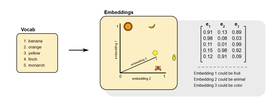
Source: Word Embeddings
What makes embeddings powerful is that the distance between vectors has meaning. If two vectors are close, the model treats them as similar. If they are far apart, the model treats them as different. This allows simple tools like distance calculations or nearest neighbor search to work well.
The same idea can be used for locations. A place on Earth is not just a coordinate; it is a combination of surrounding infrastructure, human activity, and environmental context. The geo embedding turns this complexity into a vector. Two locations that are close on the ground, or used in similar ways, can end up close in vector space. This makes location data much easier to use in clustering, similarity search, and machine learning models.
Why Use Geo Embeddings?
Geo embeddings matter because they change how geospatial data is handled from the ground up.
A single location is rarely described by just one attribute. In practice, it may be linked to imagery, climate signals, elevation, roads, population, or human activity. Working with all these layers directly is heavy and often repetitive. Geo embeddings help by compressing this rich information into a short vector that models can use easily. This becomes especially useful when working with large areas or multiple datasets, which is why embeddings are a key component in modern systems built around geospatial foundation models.
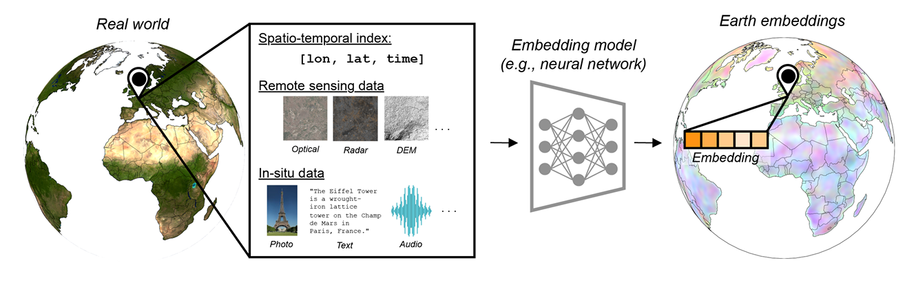
Source: Earth Embeddings: Towards AI-centric Representations of our Planet
Geo embeddings also make it easier to combine different kinds of data. Text, images, and structured features can all be tied to the same location. By representing them in a shared vector space, models can learn from these sources together instead of treating them as separate layers. This idea is used in real-world systems such as geospatially aware place embeddings, where location context improves tasks like matching and prediction.
Another important benefit is reuse. Once a location is represented as a vector, that same vector can be used again and again. It can support prediction, clustering, or similarity search without redesigning location features for every task. This reuse is the same reason vector embeddings are effective across many areas of machine learning.
Finally, geo embeddings simplify geospatial workflows. Instead of building many handcrafted features and complex preprocessing steps for each new project, users can start from a strong default representation of location and focus on the problem they actually want to solve.
At a high level, geo embeddings shift geospatial analysis from managing many disconnected layers to working with one meaningful vector per place.
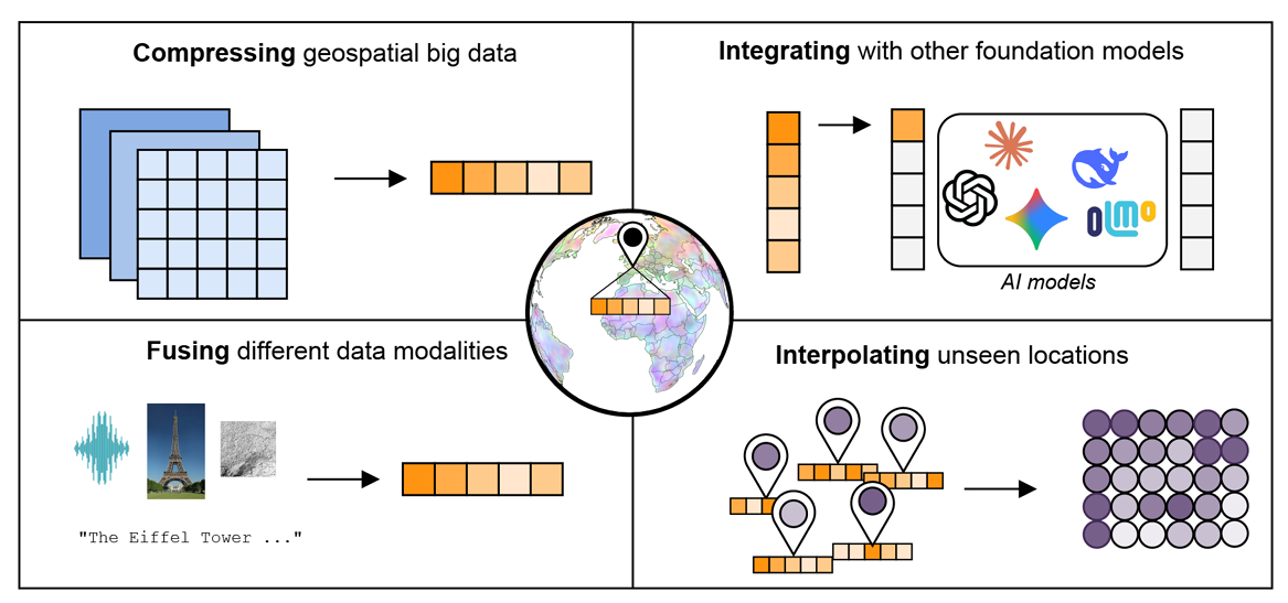
Source: Earth Embeddings: Towards AI-centric Representations of our Planet
Getting Started with Python
Let us look at a very small example with just three locations.
munich = (48.1351, 11.5820) augsburg = (48.3705, 10.8978) tokyo = (35.6762, 139.6503) |
Step 1: Real distance on Earth
Latitude and longitude do not live on a flat map. The Earth is round, so distance must be measured along its surface. The Haversine formula does exactly this. It calculates the shortest path between two points on the Earth, also called the great circle distance.
import math def haversine(lat1, lon1, lat2, lon2): r = 6371 lat1, lon1, lat2, lon2 = map(math.radians, [lat1, lon1, lat2, lon2]) dlat = lat2 - lat1 dlon = lon2 - lon1 a = math.sin(dlat / 2)**2 + math.cos(lat1) * math.cos(lat2) * math.sin(dlon / 2)**2 c = 2 * math.asin(math.sqrt(a)) return r * c |
Using this, we can compare distances between locations.
print("Munich → Augsburg (km):", round(haversine(*munich, *augsburg), 1)) print("Munich → Tokyo (km):", round(haversine(*munich, *tokyo), 1)) |
Output:
Munich → Augsburg (km): 57.0
Munich → Tokyo (km): 9369.1
This confirms what we expect. Munich is much closer to Augsburg than to Tokyo. But notice that we had to use special math just to get this right. Raw coordinates alone are not enough.
Step 2: A simple geo embedding with H3
Instead of working with distance every time, we can turn each location into a single value that already encodes proximity. H3 (global spatial indexing system developed by Uber) does this by dividing the Earth into hexagonal cells and assigning each cell a unique ID.
The resolution controls cell size. Resolution 7 is roughly city scale, which works well for simple examples.
import h3 resolution = 7 munich_h3 = h3.latlng_to_cell(*munich, resolution) augsburg_h3 = h3.latlng_to_cell(*augsburg, resolution) tokyo_h3 = h3.latlng_to_cell(*tokyo, resolution) print("Munich →", munich_h3) print("Augsburg →", augsburg_h3) print("Tokyo →", tokyo_h3) |
Output:
Munich → 871f8d7a4ffffff
Augsburg → 871f8c349ffffff
Tokyo → 872f5a363ffffff
Each location is now represented by one string. Munich and Augsburg share a similar H3 prefix, which shows that they fall into nearby hexagonal cells, while Tokyo belongs to a completely different part of the grid. This single value already captures proximity in a form that machine learning models handle much better.
This is a fixed geo embedding. It does not learn meaning from data, but it provides a clean and stable way to represent location without worrying about Earth’s curvature or inconsistent distance scaling. In the next section, we will look at embeddings that learn similarity from data, not just physical distance.
Note: While H3 is technically a geospatial index (a way to categorize space), in this context, we can think of it as a fixed embedding because it provides a stable representation of location that models can use more easily than raw coordinates.
Learning Based Geo Embeddings
Learning based geo embeddings go one step further than fixed grids like H3. H3 captures physical closeness, but many real-world problems care more about how places are used.
Instead of dividing the Earth into fixed cells, learning based methods learn location vectors from data. The idea is simple. Places that have similar attributes should have similar vectors. If two areas are used in similar ways – whether through visitor patterns, deliveries, or other activities – they should be represented close to each other in the embedding space. This way of learning places meaning from behavior appears in work on location representation learning. This idea is similar to how embeddings work in language. Words that appear in similar contexts get similar vectors. For locations, the context comes from movement and activity, such as GPS traces, check -ns, or nearby services.
The result is a vector for each location. Two places can be close in this space even if they are far apart on the map. For example, business districts in different cities can end up closer to each other than to nearby residential areas. Systems like Loc2Vec follow this approach.
These embeddings are more flexible than fixed grids, but also harder to build. For many tasks, simple spatial indexing is enough. Learning based embeddings are useful when you care about place meaning and behavior, not just distance.
Next Steps and Resources
If you want to continue learning about geo embeddings, the most important thing is to stay practical.
A good next step is to spend more time with H3. Even though it is an index, it builds the spatial intuition you need for more advanced work. Try changing the resolution and observe how cell size changes. Count points per cell, look at neighbors, and visualize results on a map. This builds intuition for how location turns into structure. The official H3 documentation is the best reference for this stage, and you do not need to read it all. Focus on indexing, resolution, and neighbors.
Once you are comfortable with fixed grids, the next step is understanding what embeddings can represent, not how to train them. A broad and readable overview is Earth Embeddings: Towards AI-centric Representations of Geospatial Data. You do not need to follow the technical details. Read it to understand what kinds of information embeddings can carry and why they are useful across many geospatial problems.
If you want to see embeddings applied to real data without building models yourself, explore how satellite data is represented as vectors in practice. Resources like Google Earth Engine’s embedding datasets show how embeddings are used for classification, regression, and similarity search at scale.
Future Outlook
Geo embeddings are already being used in real systems, not just experiments.
Open source Earth foundation models like Clay show how a single model can produce reusable Earth embeddings from multiple satellite sources. These embeddings act as a common representation for many downstream tasks instead of task-specific features.
Other projects connect space with language. SkyScript links satellite imagery and text descriptions in a shared vector space, making it possible to search for locations using natural language instead of coordinates.
Large-scale platforms are also adopting these ideas. Microsoft’s Planetary Computer uses embedding-based methods to support global environmental monitoring and similarity search across ecosystems.
Together, these projects show where the field is heading: location is becoming a vector that can be searched, compared, and reused across many systems.
Further Resources
- https://dataarmyintel.io/knowledge-article/geohash-or-h3-which-geospatial-indexing-system-should-i-use/
- https://medium.com/google-earth/ai-powered-pixels-introducing-googles-satellite-embedding-dataset-31744c1f4650
- https://www.youtube.com/watch?v=UN0vvSxQ-50
- https://www.ibm.com/think/topics/vector-embedding
Did you like this post? Read more and subscribe to our monthly newsletter!

#Contributing Writers


Next article
December is a month when maps stop being just analytical tools and start telling stories that anyone can read. From glowing cities to snow-covered landscapes, GIS and Earth Observation offer ways to explore the holiday season. Let’s take a journey across maps, satellite imagery, and even the cosmos, all through the lens of geospatial science.
Tacky Lights and Holiday Maps
For some, Christmas is about elaborate light displays. Recent Holly’s Tacky Christmas Lights map in Fairfax highlights the most colorful houses in town, turning local decorations into a living, interactive dataset. GIS enthusiasts can appreciate how simple point data and symbology transform the urban landscape into a sparkling holiday story.
Map of Tacky Christmas Lights – Source
Meanwhile, vector tile layers with Christmas-themed basemaps offer a playful twist for cartographers experimenting with holiday aesthetics. While not meant for production use, these layers demonstrate how GIS styling can be seasonally expressive, turning the world itself into a festive canvas.
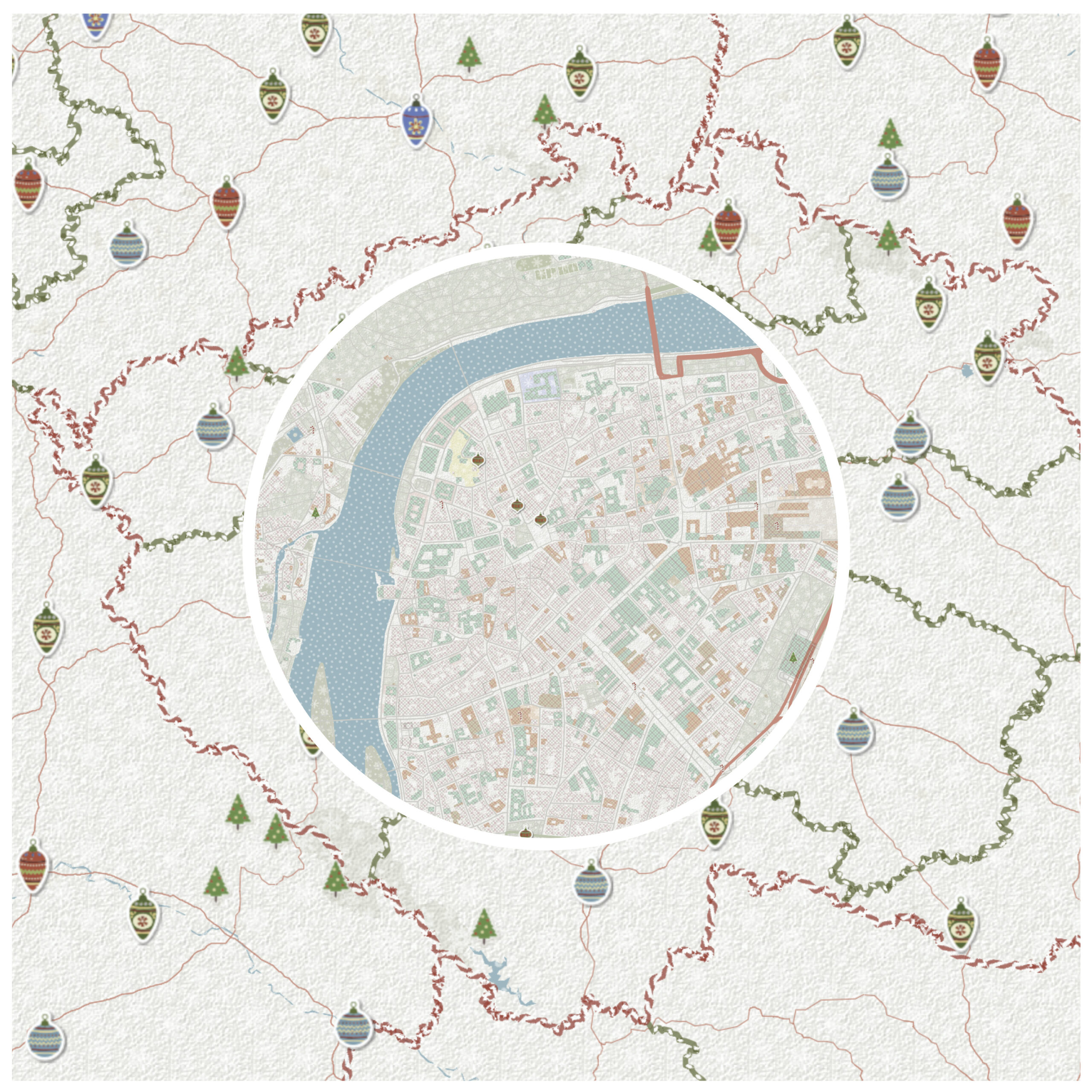
Vector Tile Christmas Basemap: A Close Look at Prague, Czech Republic
Snow, White Christmases, and Satellite Views
Nothing says winter like snow on the map. EO provides a unique perspective on seasonal extremes. MODIS imagery captured Great Britain on 7 January 2010, blanketed in snow—a satellite snapshot that makes winter tangible for anyone studying the UK from space.
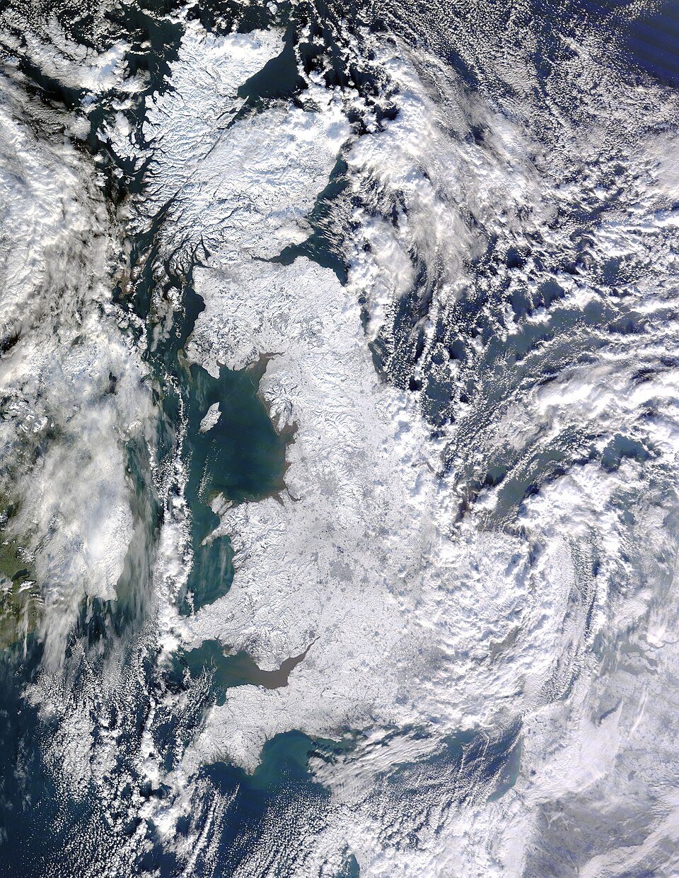
MODIS Snow Image – Great Britain, 2010
For those dreaming of a white Christmas, interactive and static maps of the United States and Europe show probabilities of snow on December 25th. These maps combine climatology, historical records, and predictive modeling, perfect examples of GIS in seasonal decision-making.
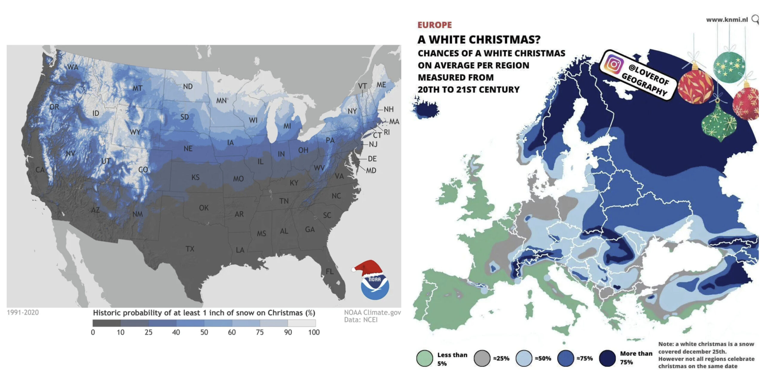
White Christmas Probability Maps – US & Europe
Christmas Trees and Lidar Landscapes
GIS also maps where traditions grow. The US hosts diverse Christmas tree farms, and maps show exactly where your festive firs originate. Lidar technology adds a modern twist, revealing the 3D structure of these farms and even individual trees with centimeter-level detail.
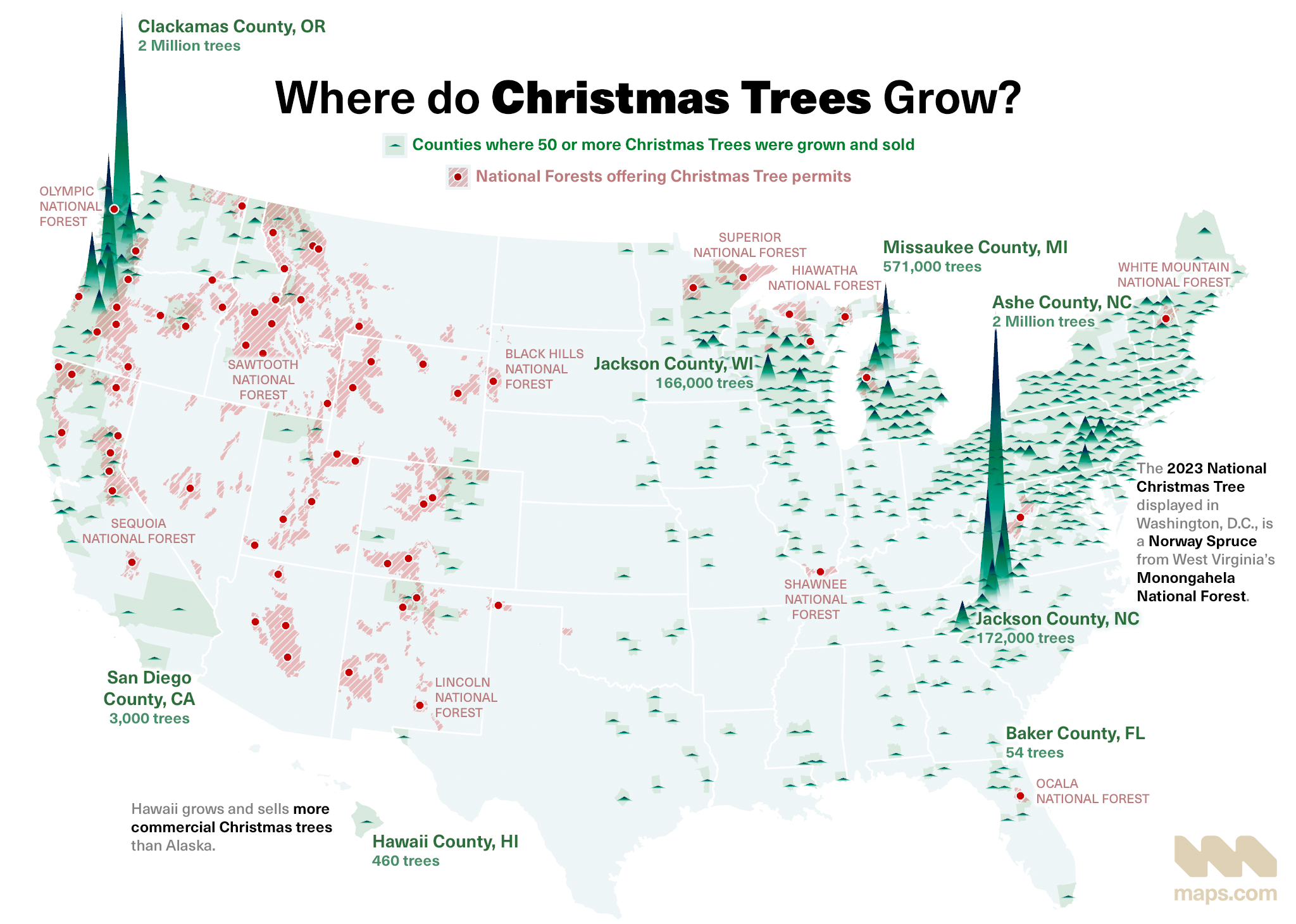
Map of Christmas Tree Farms in the US
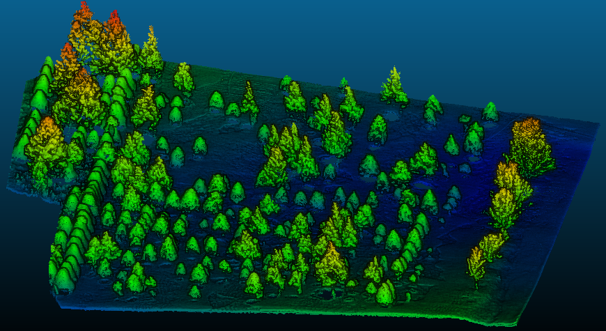
Lidar Map of a Christmas Tree Farm
Cities That Glow from Space
December nights are long, and Earth Observation satellites capture an extraordinary glow from cities around the world. NASA’s analysis “Even from Space, Holidays Shine Brightly” shows that urban areas illuminate much more intensely during the holiday season. Nighttime lights datasets offer insights not only into festivity but also into energy consumption and urban patterns.
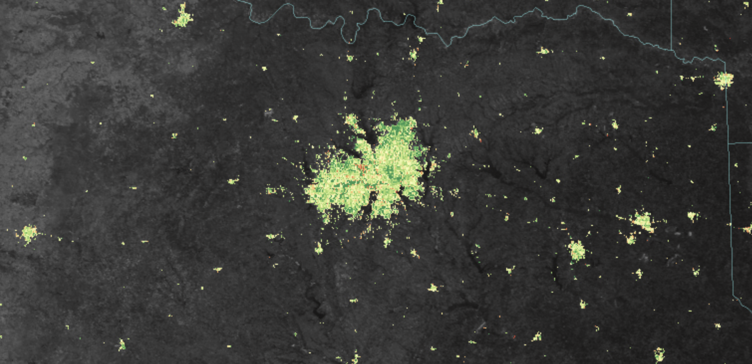
NASA EO Holiday Lights Imagery for Dallas, US. Green areas indicate places with more glow in the holiday season compared to the rest of the year
A close-up of New York City’s iconic Christmas tree in Rockefeller Center demonstrates how EO and high-resolution imaging converge with cultural geography, offering both visual delight and spatial understanding.
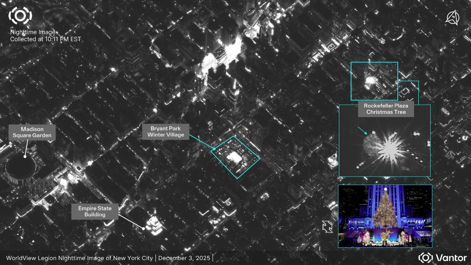
High-Detail NYC Christmas Tree Image 2025 – Source: Vantor
Mapping Holiday Folklore
Cartography has long visualized myths, and Jakub Marian’s map of European Christmas gift-bringers shows how geospatial storytelling can chart Santa, Père Noël, Krampus, and more. It’s a playful reminder that maps aren’t just about coordinates: they encode culture and history.
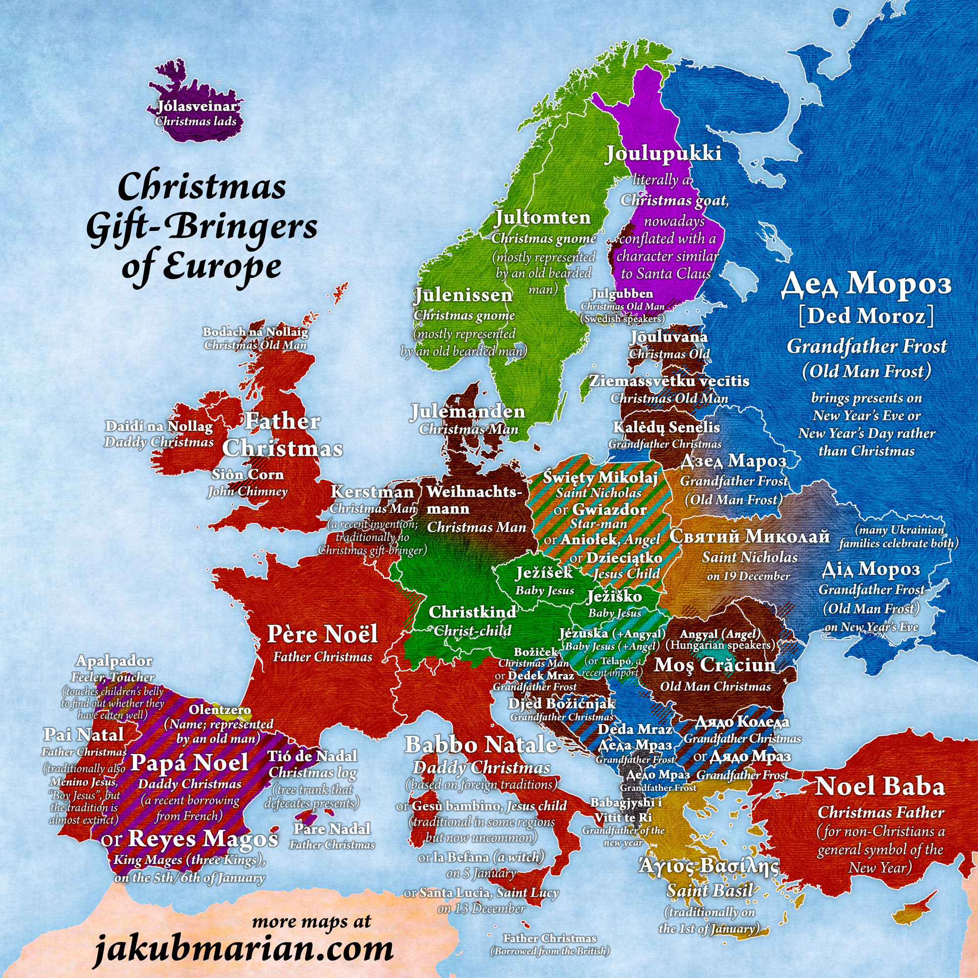
Map of Christmas Gift-Bringers in Europe – Jakub Marian
Space Christmas Tree
Even beyond our planet, the holidays inspire geospatial imagination. NASA’s “Christmas Tree Cluster” captures star formations reminiscent of festive conifers.
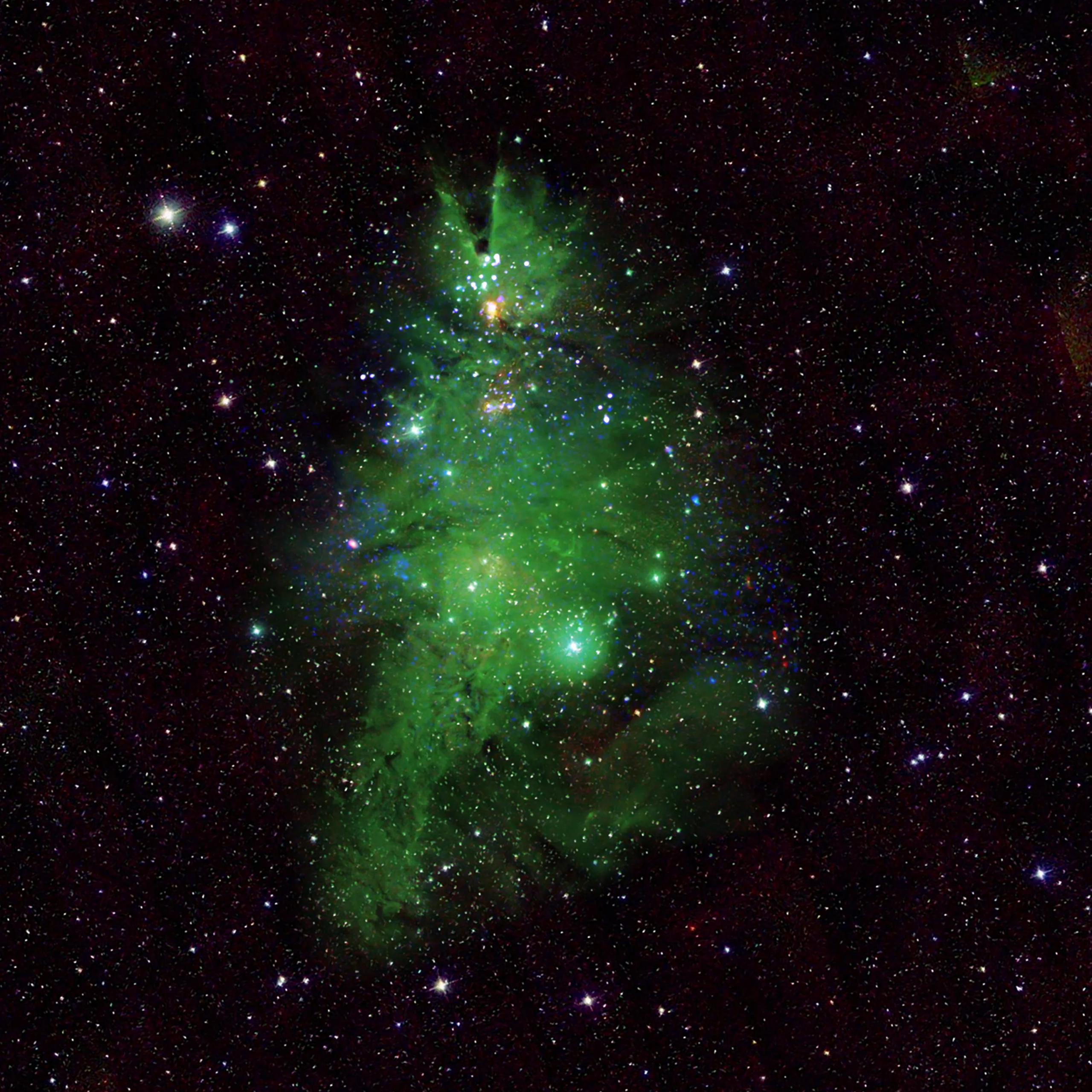
NASA Christmas Tree Cluster Image
Geospatial data touches almost every part of our lives. That’s why we love seeing it bring winter holidays to life: twinkling lights, snowy landscapes, tree farms, and even cities glowing from space. GIS and Earth Observation let us experience the holidays in ways we never thought possible.

Wishing Merry Christmas to all, from Geoawesome!
Did you like this post? Read more and subscribe to our monthly newsletter!

